Training SchNet on rMD17 (ethanol)

This notebook trains the xnn SchNet from scratch on the paper’s own benchmark task: predicting the energies and forces of a molecular-dynamics trajectory of a small organic molecule, ethaol. The dataset is downloaded in seconds through the xnn hub and the model reproduces the SchNet manuscript’s headline at small scale:

• Training on joint energy + force training with the paper’s loss weighting (\(\rho = 0.01\)): forces are calculated via autograd through the ForceStressOutput wrapper the Trainer adds (Thus, the model is energy-conserving by construction).

• The trainer’s loggers: every epoch’s losses and MAE/RMSE, averaged over the whole training and validation sets, go to metrics.csv which is used to draw the learning curves.

• An energy/force parity plot vs DFT labels on held-out conformations is created.

• A smooth 1-D potential-energy scan, the property that continuous filters + shifted softplus can calculate over discretized approaches.

The model implemented here is based on the paper’s architecture (\(F = 64\), \(T = 3\), Gaussian RBFs every 0.1 Å with \(\gamma = 10\) Å\(^{-2}\)). The implementation is verified against the manuscripts’ equations block by block in examples/fidelity_checks/schnet_verification.ipynb.

Note: Run with this notebook with xnn kernel (which uses the GPU when available). See the documentation or pyproject.toml for installation instructions.

0. Setup and data

import time, warnings
warnings.filterwarnings("ignore")
import numpy as np
import torch
import matplotlib.pyplot as plt

torch.set_default_dtype(torch.float64)
torch.manual_seed(0)

from xnn.common.data import load_dataset

# The paper trains without a distance cutoff -- its RBF grid just ends beyond
# every pair distance. Ethanol spans < 5 A, so a 10 A radius reproduces that
# no-cutoff setting (complete graph) with a matching 0.1 A RBF grid
CUTOFF, N_RBF = 10.0, 101

# Load the RMD17 ethanol dataset, which is small enough to fit in memory
splits = load_dataset("rmd17", molecule="ethanol", n_train=1000, n_test=500, quiet=True)

# Split the dataset into training and testing sets
train_structs, test_structs = splits["train"], splits["test"]

# Count the number of atoms in the first training structure
N_ATOMS = len(train_structs[0]["atomic_numbers"])

# Print the number of training and testing structures, as well as the number of
# atoms per molecule
print(
    f"train {len(train_structs)}  test {len(test_structs)}  "
    f"atoms/molecule {N_ATOMS}"
)

train 1000  test 500  atoms/molecule 9

1. Per-atom energy standardization

SchNet inherits the Deep Tensor Neural Netrowk (DTNN)’s output convention: the network predicts a standardized per-atom energy \(\hat E_i\), and the final contribution is

\[E_i = E_\sigma \hat E_i + E_\mu\]

where \(E_\mu\) and \(E_\sigma\) denote the mean and standard deviation of the energy per atom over the training set, respectively. With the zero-initialized output head, the model’s first prediction is exactly the training-set mean which may provide a good starting point for the training.

# Compute the mean and standard deviation of the energy per atom in the training
# set
E_train = np.array([s["energy"] for s in train_structs])
E_SHIFT = float(E_train.mean() / N_ATOMS)     # E_mu   (eV / atom)
E_SCALE = float(E_train.std() / N_ATOMS)      # E_sigma (eV / atom)

# Print the mean and standard deviation of the energy per atom, as well as the
# total-energy spread of the trajectory
print(f"E_mu = {E_SHIFT:.4f} eV/atom   E_sigma = {E_SCALE:.5f} eV/atom")
print(f"(total-energy spread of the trajectory: {E_train.std():.3f} eV)")

E_mu = -467.7363 eV/atom   E_sigma = 0.01981 eV/atom
(total-energy spread of the trajectory: 0.178 eV)

2. Build SchNet and train on energies + forces

The SchNet manuscript’s combined loss is

\[\ell = \rho\,\|E - \hat E\|^2 + \frac{1}{n}\sum_i \|F_i + \partial\hat E/\partial R_i\|^2\]

with \(\rho = 0.01\). The xnn trainer normalizes the energy term per atom so energy_weight=1, force_weight=1 gives an effective energy/force ratio of \(1/n^2 = 1/81 \approx 0.012\), the paper’s \(\rho\). The trainer section of the config picks the best.pt and the plateau scheduler follows the validation loss and the error metrics that are being computed. The loggers decide where the metrics will be stored/printed: a CSVLogger keeps every epoch in runs/schnet_rmd17/metrics.csv, and a ConsoleLogger subclass prints to the standard output interface every 50th epoch.

from torch.utils.data import Subset
from xnn.common.data import AtomicDataset
from xnn.common.config import (
    Config,
    ModelConfig,
    DataConfig,
    OptimConfig,
    TrainerConfig,
)
from xnn.common.train import ConsoleLogger, CSVLogger, Trainer

# Training hyperparameters
EPOCHS, BS, LR = 300, 32, 1e-3

# Create the training and testing datasets using the AtomicDataset class, with
# the specified cutoff distance
train_ds = AtomicDataset(train_structs, CUTOFF)
test_ds = AtomicDataset(test_structs, CUTOFF)

# Create a validation set of 100 structures from the training set, and use the
# remaining structures for training
n_val = 100
val_idx = list(range(n_val))
tr_idx = list(range(n_val, len(train_ds)))

# Create a configuration object for the SchNet model, specifying the model
# architecture, data parameters, optimization settings, and output directory
cfg = Config(
    model=ModelConfig(
        name="schnet",
        cutoff=CUTOFF,
        n_features=64,
        n_interactions=3,
        n_rbf=N_RBF,
        extra={"gamma": 10.0, "energy_shift": E_SHIFT, "energy_scale": E_SCALE},
    ),
    data=DataConfig(cutoff=CUTOFF, batch_size=BS),
    optim=OptimConfig(
        lr=LR, epochs=EPOCHS, energy_weight=1.0, force_weight=1.0, scheduler="plateau"
    ),
    trainer=TrainerConfig(monitor="val/loss", metrics=["mae", "rmse"]),
    output_dir="runs/schnet_rmd17",
)

class EveryNEpochs(ConsoleLogger):
    """Prints the epoch lines of every n-th epoch and the test result."""

    def __init__(self, n):
        super().__init__()
        self.n = n

    def log_metrics(self, metrics, step):
        if "epoch" not in metrics or (metrics["epoch"] + 1) % self.n == 0:
            super().log_metrics(metrics, step)


# Every epoch goes to runs/schnet_rmd17/metrics.csv, every 50th to the screen
csv_logger = CSVLogger()
trainer = Trainer(
    cfg,
    Subset(train_ds, tr_idx),
    Subset(train_ds, val_idx),
    test_ds,
    logger=[csv_logger, EveryNEpochs(50)],
)

# Count the number of parameters in the SchNet model and print it along with the
# device being used for training
n_params = sum(p.numel() for p in trainer.module.parameters())
print(f"SchNet parameters: {n_params:,}  |  device: {trainer.device}")

# Train the SchNet model for the specified number of epochs and print the total
# training time
t0 = time.time()
metrics = trainer.fit()
print(f"trained {EPOCHS} epochs in {time.time()-t0:.0f}s")

SchNet parameters: 78,117  |  device: cuda
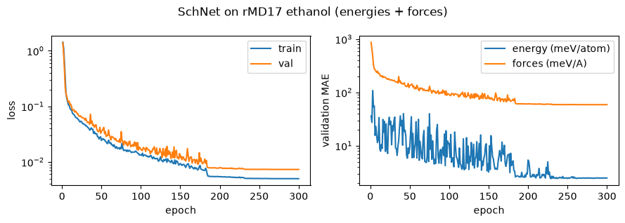
epoch   49 | train loss 2.4335e-02 (energy 2.068e-04, force 2.413e-02) | val loss 3.5942e-02 (energy 1.151e-04, force 3.583e-02)
          val mae: energy 9.378e-03, forces 1.339e-01 | rmse: energy 1.073e-02, forces 1.893e-01
epoch   99 | train loss 1.3431e-02 (energy 1.310e-04, force 1.330e-02) | val loss 1.6855e-02 (energy 1.426e-04, force 1.671e-02)
          val mae: energy 1.090e-02, forces 9.006e-02 | rmse: energy 1.194e-02, forces 1.293e-01
epoch  149 | train loss 9.3349e-03 (energy 6.929e-05, force 9.266e-03) | val loss 1.1998e-02 (energy 1.633e-05, force 1.198e-02)
          val mae: energy 3.217e-03, forces 7.771e-02 | rmse: energy 4.041e-03, forces 1.095e-01
epoch  199 | train loss 5.4274e-03 (energy 2.104e-05, force 5.406e-03) | val loss 7.8981e-03 (energy 3.643e-05, force 7.862e-03)
          val mae: energy 5.387e-03, forces 6.109e-02 | rmse: energy 6.036e-03, forces 8.867e-02
epoch  249 | train loss 5.0365e-03 (energy 9.388e-06, force 5.027e-03) | val loss 7.3526e-03 (energy 9.181e-06, force 7.343e-03)
          val mae: energy 2.431e-03, forces 5.914e-02 | rmse: energy 3.030e-03, forces 8.569e-02
epoch  299 | train loss 4.9968e-03 (energy 9.328e-06, force 4.987e-03) | val loss 7.3143e-03 (energy 9.284e-06, force 7.305e-03)
          val mae: energy 2.480e-03, forces 5.891e-02 | rmse: energy 3.047e-03, forces 8.547e-02
test loss 6.9461e-03 (energy 1.131e-05, force 6.935e-03)
          test mae: energy 2.591e-03, forces 5.914e-02 | rmse: energy 3.364e-03, forces 8.328e-02
trained 300 epochs in 649s

3. Learning curves

The loss and the validation MAEs of every epoch, read back from metrics.csv (the energy MAE is per atom), can be plotted as shown below

import csv

# One row per epoch, then one row with the test metrics
with open(csv_logger.path) as f:
    rows = [r for r in csv.DictReader(f) if r["epoch"]]

# Extract the data for plotting
col = lambda key: np.array([float(r[key]) for r in rows])
epoch = col("epoch") + 1

# Plot the training and validation loss
fig, (a1, a2) = plt.subplots(1, 2, figsize=(9, 3.2))
a1.plot(epoch, col("train/loss"), label="train")
a1.plot(epoch, col("val/loss"), label="val")
a1.set_yscale("log")
a1.set_xlabel("epoch")
a1.set_ylabel("loss")
a1.legend()
a2.plot(epoch, col("val/energy_mae") * 1e3, label="energy (meV/atom)")
a2.plot(epoch, col("val/forces_mae") * 1e3, label="forces (meV/A)")
a2.set_yscale("log")
a2.set_xlabel("epoch")
a2.set_ylabel("validation MAE")
a2.legend()
fig.suptitle("SchNet on rMD17 ethanol (energies + forces)")
fig.tight_layout()
fig.savefig("schnet_loss_curves.png", dpi=110)
plt.show()

4. Energy & force parity vs DFT

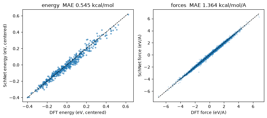
We load best.pt, the weights of the epoch with the lowest validation loss (the checkpoint schnet_ethanol_md.ipynb runs), predict on the 500 held-out conformations and compare to the reference DFT values. The MAEs are in kcal/mol with the energy error per molecule in order to be consist with the SchNet manuscript.

For comparison: SchNet, trained on \(N = 1000\) MD17 ethanol conformations, reaches MAE of 0.08 kcal/mol (energy) and 0.39 kcal/mol/Å (forces) in Table 2 of the SchNet manuscript, with \(\approx\) 10x longer training and learning-rate decay. This 300-epoch run lands within a few times those numbers (sub-kcal/mol energies).

from torch.utils.data import DataLoader
from xnn.common.data import collate
from xnn.common.models.hub import from_pretrained

# Set the device to the one used by the trainer
device = str(trainer.device)

# Load the best model checkpoint from the training run and set it to evaluation
# mode
model = from_pretrained("runs/schnet_rmd17/best.pt", device=device).eval()

# Define the conversion factor from electron volts to kilocalories per mole
EV2KCAL = 23.060541945329334

# Evaluate the model on the test dataset and compute the predicted and reference
# energies and forces
E_pred, E_ref, F_pred, F_ref = [], [], [], []
for batch in DataLoader(test_ds, batch_size=50, collate_fn=collate):
    batch = batch.to(device)
    out = model(batch)
    E_pred.append(out["energy"].detach().cpu().numpy())
    E_ref.append(batch.energy.detach().cpu().numpy())
    F_pred.append(out["forces"].detach().cpu().numpy())
    F_ref.append(batch.forces.detach().cpu().numpy())
E_pred, E_ref = np.concatenate(E_pred), np.concatenate(E_ref)
F_pred, F_ref = np.concatenate(F_pred), np.concatenate(F_ref)

# Compute the mean absolute error (MAE) and root mean square error (RMSE) for
# both energies and forces, and print the results in both meV and kcal/mol units
e_mae = np.abs(E_pred - E_ref).mean()
f_mae = np.abs(F_pred - F_ref).mean()
e_rmse = np.sqrt(np.mean((E_pred - E_ref) ** 2))
f_rmse = np.sqrt(np.mean((F_pred - F_ref) ** 2))
print(f"energy MAE : {e_mae*1e3:6.2f} meV    ({e_mae*EV2KCAL:.3f} kcal/mol)")
print(f"force  MAE : {f_mae*1e3:6.2f} meV/A  ({f_mae*EV2KCAL:.3f} kcal/mol/A)")
print(f"energy RMSE: {e_rmse*1e3:6.2f} meV    ({e_rmse*EV2KCAL:.3f} kcal/mol)")
print(f"force  RMSE: {f_rmse*1e3:6.2f} meV/A  ({f_rmse*EV2KCAL:.3f} kcal/mol/A)")

energy MAE :  23.62 meV    (0.545 kcal/mol)
force  MAE :  59.15 meV/A  (1.364 kcal/mol/A)
energy RMSE:  30.68 meV    (0.707 kcal/mol)
force  RMSE:  83.28 meV/A  (1.921 kcal/mol/A)

# Plot the parity between the predicted and reference energies and forces, with
# the mean absolute error (MAE) displayed in the titles 
fig, (a1, a2) = plt.subplots(1, 2, figsize=(9, 4))
a1.scatter(E_ref - E_ref.mean(), E_pred - E_ref.mean(), s=8, alpha=0.5)
lim = np.array([(E_ref - E_ref.mean()).min(), (E_ref - E_ref.mean()).max()])
a1.plot(lim, lim, "k--", lw=1)
a1.set_xlabel("DFT energy (eV, centered)")
a1.set_ylabel("SchNet energy (eV, centered)")
a1.set_title(f"energy  MAE {e_mae*EV2KCAL:.3f} kcal/mol")
a2.scatter(F_ref.ravel(), F_pred.ravel(), s=3, alpha=0.2)
lim = np.array([F_ref.min(), F_ref.max()])
a2.plot(lim, lim, "k--", lw=1)
a2.set_xlabel("DFT force (eV/A)"); a2.set_ylabel("SchNet force (eV/A)")
a2.set_title(f"forces  MAE {f_mae*EV2KCAL:.3f} kcal/mol/A")
fig.tight_layout()
fig.savefig("schnet_parity.png", dpi=110)
plt.show()

5. A smooth 1-D potential-energy scan

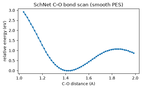
One of the reasons behind creating a continuous filter in SchNet is having a smooth, differentiable potential energy surface (the paper’s Fig. 1 contrasts this with the jagged surface a discretized filter produces). We stretch the C-O bond of a test geometry and evaluate the trained SchNet along the scan through its ASE calculator: a smooth single-well curve is what enables stable geometry optimization and MD.

from ase import Atoms
from xnn.common.deploy import XNNCalculator

# Create an ASE calculator using the trained SchNet model, with the specified
# cutoff distance and device
calc = XNNCalculator(model, cutoff=CUTOFF, device=device)

# Extract the atomic numbers and positions of the first test structure, and
# create an ASE Atoms object with the SchNet calculator
s = test_structs[0]
atoms = Atoms(numbers=s["atomic_numbers"], positions=s["pos"], calculator=calc)
Z, pos0 = atoms.numbers, atoms.positions.copy()

# Ethanol: stretch the C-O bond (the O and the nearest C)
O = int(np.flatnonzero(Z == 8)[0])
Cs = np.flatnonzero(Z == 6)
C = int(Cs[np.linalg.norm(pos0[Cs] - pos0[O], axis=1).argmin()])
axis = pos0[O] - pos0[C]
r0 = float(np.linalg.norm(axis))
axis /= r0

# Perform a bond scan by varying the C-O distance and computing the potential
# energy at each distance using the SchNet calculator. The energies are then
# shifted so that the minimum energy is zero
scan = np.linspace(-0.35, 0.6, 60)
energies = []
for dr in scan:
    pos = pos0.copy(); pos[O] += dr * axis
    atoms.positions = pos
    energies.append(atoms.get_potential_energy())
energies = np.array(energies) - min(energies)

# Plot the potential energy surface (PES) of the C-O bond scan, with the C-O
# distance on the x-axis and the relative energy on the y-axis
fig, ax = plt.subplots(figsize=(5, 3.2))
ax.plot(r0 + scan, energies, "o-", ms=3)
ax.set_xlabel("C-O distance (A)"); ax.set_ylabel("relative energy (eV)")
ax.set_title("SchNet C-O bond scan (smooth PES)")
fig.tight_layout()
fig.savefig("schnet_bond_scan.png", dpi=110)
plt.show()

Summary

• The xnn SchNet reproduces the SchNet manuscript’s results on the rMD17 ethanol dataset, achieving sub-kcal/mol accuracy in energy and force predictions.

• The model’s continuous filter architecture allows for smooth potential energy surfaces, which is crucial for stable geometry optimization and molecular dynamics simulations.

• The training process, including energy and force loss weighting, learning rate scheduling, and logging, is effectively managed by the xnn Trainer, demonstrating the framework’s capability for handling complex machine learning tasks in computational chemistry.

References

• Schütt et al., SchNet: A continuous-filter convolutional neural network for modeling quantum interactions arXiv.1706.08566 (2017)

• Schütt et al., SchNet: A deep learning architecture for molecules and materials, J. Chem. Phys. 148, 241722 (2018)