
2. Lesson 01b: Group Representations#
What you will learn
What a group representation is and why the homomorphism property, \(D(g_1 g_2) = D(g_1)\,D(g_2)\), is exactly what a network layer needs to know about its data.
What Reducible and irreducible representations are and how a \(3\times 3\) tensor decomposes.
The irreducible representations (irreps) of \(SO(3)\), which are labeled by \(l = 0, 1, 2, \dots\) with dimension \(2l+1\). Their matrix representations are the Wigner D-matrices (
o3.wigner_D).Numerical verification of the homomorphism property and the Schur orthogonality relations
The visualization of the block-diagonal structure of a reducible representation
Parity, the \(O(3) = SO(3) \times \{\mathbb{1}, P\}\) group, and why a Cartesian 3-vector is its irrep \((l{=}1,\ \text{odd})\)
Prerequisites:
Lesson 01a and/or
Basic knowledge of groups: \(SO(3) \subset O(3) \subset E(3)\)
The definition of equivariance
import sys
sys.path.insert(0, "..")  # Make course_utils importable

import matplotlib.pyplot as plt
import numpy as np
import torch
import e3nn
from e3nn import o3

torch.set_default_dtype(torch.float64)  # float64 so representation identities hold to ~1e-15
torch.manual_seed(0)
np.random.seed(0)
device = torch.device("cuda" if torch.cuda.is_available() else "cpu")
print(f"torch {torch.__version__} | device: {device}")
print(f"e3nn {e3nn.__version__}")
torch 2.7.1+cu126 | device: cuda
e3nn 0.6.0
2.1. What is a representation?#
In Lesson 01a the definition of equivariance, \(f(D_X(g)x) = D_Y(g)f(x)\), used \(D(g)\) matrices that describe “how the data transforms”. Those matrices cannot be arbitrary: they must compose the way the group does. Quoting Geiger & Smidt, e3nn: Euclidean Neural Networks arXiv.2207.09453 (2021):
For a given group \(G\), a function \(D: G \to \mathbb{R}^{d \times d}\) that maps each element of the group to a \(d \times d\) matrix is a representation iff it follows the structure of the group:
(1)\[ D(e) = \mathbb{1}, \qquad \text{and} \qquad D(g_1 g_2) = D(g_1)\, D(g_2) \qquad \forall\, g_1, g_2 \in G. \]
The vector space \(\mathbb{R}^d\) the matrices act on is the carrier space: it is where our data (features) live. Three representations of \(SO(3)\) we already know:
the trivial representation, \(D(R) = 1\) on \(\mathbb{R}^1\) — scalars;
the vector representation, \(D(R) = R\) on \(\mathbb{R}^3\) — positions, forces;
the tensor representation, \(D(R) = R \otimes R\) on \(\mathbb{R}^9\) where \(x \mapsto R\,x\,R^\top\) and \(\otimes\) denotes the Kronecker producton.
In the third case, flattening \(x\) to \(\mathrm{vec}(x) \in \mathbb{R}^9\) and transforming it with \(D(R)\), i.e., \(D(R)\,\mathrm{vec}(x)\) is equivalent to \(\mathrm{vec}(R\,x\,R^\top)\). Let’s verify this numerically.
# Verify the homomorphism property D(g1 g2) = D(g1) D(g2) for the 9-dim tensor rep
R1, R2 = o3.rand_matrix(), o3.rand_matrix()

# The tensor representation is D(R) = R kron R, where kron is the Kronecker product
D = lambda R: torch.kron(R, R)

# Verify the homomorphism property D(R1 R2) = D(R1) D(R2)
hom_err = (D(R1 @ R2) - D(R1) @ D(R2)).abs().max()
print(f"tensor rep  (d=9):  |D(R1 R2) - D(R1) D(R2)| = {hom_err:.2e}")

# ... and, trivially, for the vector rep D(R) = R (the homomorphism is R1 @ R2 itself)
x = torch.randn(3, 3)                       # a rank-2 tensor, transformed in two ways:
lhs = (D(R1) @ x.flatten()).reshape(3, 3)   # via flattening x and the 9 x 9 matrix D(R1)
rhs = R1 @ x @ R1.T                         # or via the 3 x 3 matrix R1 and the original x (3, 3)
print(f"|vec(R x R^T) - (R kron R) vec(x)|           = {(lhs - rhs).abs().max():.2e}")
tensor rep  (d=9):  |D(R1 R2) - D(R1) D(R2)| = 1.67e-16
|vec(R x R^T) - (R kron R) vec(x)|           = 2.78e-16
2.2. Reducible vs. irreducible representations#
The 9-dimensional tensor representation is wasteful because it contains and can be reduced to smaller representations. Geiger & Smidt, e3nn: Euclidean Neural Networks arXiv.2207.09453 (2021) mentions:
An irreducible representation (irrep) is a representation that does not contain a smaller representation in it.
So, what does “contains” mean in the present context? It means there is a subspace in the current 9-dimentional tensor representation that transforms only within itself and among its members. For a \(3\times 3\) tensor \(x\) under the transformation \(x \mapsto RxR^\top\):
the trace \(\mathrm{Tr}(x)\) is a single number that never mixes with the remaining elements of the tensor: the trace, therefore, creates a 1-dimensional invariant subspace (a scalar, \(l = 0\));
the antisymmetric part \(\tfrac{1}{2}(x - x^\top)\) has 3 independent components that mix only among themselves (\(l = 1\); it is equivalent to a vector via \(a_k = \tfrac{1}{2}\epsilon_{ijk} x_{ij}\));
the symmetric traceless part has \(5\) components that mix only among themselves (\(l = 2\)).
So, \(9 = 1 + 3 + 5\): the tensor representation is reducible, and in the right basis, its matrix representation becomes block-diagonal with \(l=0\), \(1\) and \(2\) blocks. As such, it should not be surprising to see that the irreps of groups such as \(SO(3)\) are indexed by \(l = 0, 1, 2, \dots\). Each irrep, labeled by \(l\) has a dimension of \(2l + 1\). The Wigner D-matrices, \(D^{(l)}(g) \in \mathbb{R}^{(2l+1) \times (2l+1)}\), are the representation matrices of the \(l\)-irreps.
Note: The Wigner D-matrices are unitary matrices. However, The e3nn works in a real basis, so the representation matrices of the \(l\)-irreps (or Wigner D-matrices) become real orthogonal matrices.
Every finite-dimensional representation of \(SO(3)\) decomposes into a direct sum of irreps. As such, irreps are the “prime numbers” of representation theory, and they will be the native data types of every network in this course.
Let’s check out the Wigner D-matrices for various \(l\) values and verify their dimensions. First, we need to create a random rotation matrix \(R\) and convert it to Euler angles, \((\alpha, \beta, \gamma)\) to compute the Wigner D-matrices. You can use e3nn’s o3.wigner_D(l, alpha, beta, gamma) to calculate the Wigner D-matrix with Euler angles.
# A rotation matrix R is converted to angles with o3.matrix_to_angles(R).
R = o3.rand_matrix()

# D^(l)(R): the l-irrep matrix of the rotation R
def D_l(l, R):
    return o3.wigner_D(l, *o3.matrix_to_angles(R))

# Create a random rotation matrix R and compute the Wigner D-matrices for l = 0, 1, 2, 3
for l in range(4):
    Dl = D_l(l, R)
    print(f"l = {l}:  D^(l) shape {tuple(Dl.shape)}   (dimension 2l+1 = {2*l+1})")
l = 0:  D^(l) shape (1, 1)   (dimension 2l+1 = 1)
l = 1:  D^(l) shape (3, 3)   (dimension 2l+1 = 3)
l = 2:  D^(l) shape (5, 5)   (dimension 2l+1 = 5)
l = 3:  D^(l) shape (7, 7)   (dimension 2l+1 = 7)
Having calculated the Wigner D-matrices, we can check their homomorphism property, expressed by
as well as their unitarity (orthogonality in the real basis), expressed by
# Numerical checks, for each l: homomorphism, orthogonality, identity

# Create two random rotation matrices R1 and R2, and the identity matrix I3
R1, R2, I3 = o3.rand_matrix(), o3.rand_matrix(), torch.eye(3)

# Print the header for the numerical checks
print(f"{'l':>2} {'|D(R1 R2)-D(R1)D(R2)|':>22} {'|D^T D - 1|':>14} {'|D(1)-1|':>10}")

# Perform the numerical checks for l = 0, 1, 2, 3
for l in range(4):
    # Compute the maximum absolute errors for homomorphism, orthogonality, and identity
    hom  = (D_l(l, R1 @ R2) - D_l(l, R1) @ D_l(l, R2)).abs().max()

    # Here, l=l' and R1 is a rotation matrix, so D_l(l, R1) should be orthogonal: D^T D = 1
    orth = (D_l(l, R1).T @ D_l(l, R1) - torch.eye(2 * l + 1)).abs().max()
    idn  = (D_l(l, I3) - torch.eye(2 * l + 1)).abs().max()
    print(f"{l:>2} {hom:>22.2e} {orth:>14.2e} {idn:>10.2e}")
 l  |D(R1 R2)-D(R1)D(R2)|    |D^T D - 1|   |D(1)-1|
 0               0.00e+00       0.00e+00   0.00e+00
 1               1.11e-15       1.78e-15   0.00e+00
 2               4.00e-15       4.66e-15   0.00e+00
 3               1.20e-14       6.88e-15   0.00e+00
All identities hold to float64 round-off: each \(D^{(l)}\) is a genuine representation (homomorphism + identity), and its matrices are orthogonal, \(D^{(l)}(R)^\top D^{(l)}(R) = \mathbb{1}\): rotating features never changes their norm. This is why deep equivariant networks don’t suffer from features blowing up under rotation.
2.2.1. Schur orthogonality: different irreps are perpendicular functions#
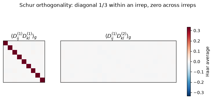
According to the classical Schur orthogonality relation, applied to the Wigner D-matrices and \(SO(3)\) group,
the irreps of \(SO(3)\) are orthogonal to each other. Here, \(d\mu(g)\) is the (normalized) Haar measure: the unique rotation-invariant way to average over the group, which is exactly what o3.rand_matrix samples from.
Let us verify the Schur orthogonality by Monte Carlo. Here, we assume \(\mu \approx g\) and average the products of Wigner-D entries over many random rotations.
# Set the number of random rotations to sample for the Monte Carlo verification
# of Schur orthogonality
n = 20_000

# Haar-random rotations, batched
angles = o3.matrix_to_angles(o3.rand_matrix(n))

# rows: vec of D^(1)(g)
D1 = o3.wigner_D(1, *angles).reshape(n, 9)
D2 = o3.wigner_D(2, *angles).reshape(n, 25)

# For l=l'=1, (2l+1, 2l'+1) = (9, 9)
# expect  1/(2l+1) * identity = I/3
gram_11 = D1.T @ D1 / n

# For l=1, l'=2, (2l+1, 2l'+1) = (9, 25)
# expect  0 (different irreps)
gram_12 = D1.T @ D2 / n

# Print the maximum absolute errors for the same irrep (l=1,l=1) and cross irrep (l=1,l=2)
print(f"same irrep  (l=1,l=1): max |gram - I/3| = {(gram_11 - torch.eye(9)/3).abs().max():.1e}"
      f"   (Monte-Carlo error ~ 1/sqrt(n) = {n ** -0.5:.1e})")
print(f"cross irrep (l=1,l=2): max |gram|       = {gram_12.abs().max():.1e}")

# Plot the Gram matrices for the same irrep (l=1,l=1) and cross irrep (l=1,l=2)
fig, axes = plt.subplots(1, 2, figsize=(9, 3.6), width_ratios=[9, 25])

for ax, g, title in [(axes[0], gram_11, r"$\langle D^{(1)}_{ij} D^{(1)}_{kl}\rangle_g$"),
                     (axes[1], gram_12, r"$\langle D^{(1)}_{ij} D^{(2)}_{kl}\rangle_g$")]:
    im = ax.matshow(g, cmap="RdBu_r", vmin=-1/3, vmax=1/3)
    ax.set_title(title)
    ax.set_xticks([])
    ax.set_yticks([])

fig.colorbar(im, ax=axes, shrink=0.8, label="Haar average")
fig.suptitle("Schur orthogonality: diagonal 1/3 within an irrep, zero across irreps", y=1.02);
same irrep  (l=1,l=1): max |gram - I/3| = 5.2e-03   (Monte-Carlo error ~ 1/sqrt(n) = 7.1e-03)
cross irrep (l=1,l=2): max |gram|       = 5.1e-03
2.3. Reducible representations are block-diagonal: Visualizing the direct sum#
If a carrier space is a direct sum of irreps, say \(l{=}0 \oplus l{=}1 \oplus l{=}2\) (dimension \(1 + 3 + 5 = 9\)), then in the irrep basis, every representation matrix is block-diagonal:
In e3nn, this direct sum is written as the irreps string "1x0e + 1x1o + 1x2e" (multiplicity × irrep; the e/o parity labels are explained in the next section; Lesson 02a fully dissects the notation). o3.Irreps.D_from_matrix builds the whole block-diagonal matrix from a \(3\times 3\) orthogonal matrix. Let’s see that in action by plotting the block-diagonal structure of a reducible representation:
# Create a reducible representation as a direct sum of irreps: 0e + 1o + 2e
irreps = o3.Irreps("1x0e + 1x1o + 1x2e")
print(f"irreps = {irreps},  total dimension = {irreps.dim}")

# Create a random rotation matrix R and compute the block-diagonal representation D(g)
R = o3.rand_matrix()

# (9, 9) block-diagonal: D^0 (+) D^1 (+) D^2
D = irreps.D_from_matrix(R)

# Plot the block-diagonal structure of the reducible representation D(g)
fig, ax = plt.subplots(figsize=(4.6, 4.6))
ax.matshow(D, cmap="RdBu_r", vmin=-1, vmax=1)

for b in (1, 4):
    # block boundaries after dims 1 and 1+3
    ax.axhline(b - 0.5, color="k", lw=0.8); ax.axvline(b - 0.5, color="k", lw=0.8)

ax.set_xticks([0, 2, 6]); ax.set_xticklabels(["0e", "1o", "2e"])
ax.set_yticks([0, 2, 6]); ax.set_yticklabels(["0e", "1o", "2e"])
ax.set_title(r"$D(g)$ for irreps $0e \oplus 1o \oplus 2e$: block-diagonal")

blocks = [D[:1, :1], D[1:4, 1:4], D[4:, 4:]]
print("blocks match the individual Wigner matrices:",
      max((b - D_l(l, R)).abs().max().item() for l, b in enumerate(blocks)))
irreps = 1x0e+1x1o+1x2e,  total dimension = 9
blocks match the individual Wigner matrices: 0.0
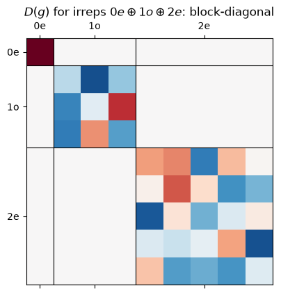
Everything outside the blocks is exactly zero. Under rotation, scalar components (\(l=0\)) never mix into vector components (\(l=1\)), and vectors never mix into \(l=2\) components, and so on. An equivariant network is precisely a network whose features carry such a block structure and whose layers are constrained to respect it.
2.4. Parity: from \(SO(3)\) to \(O(3)\)#
As we saw in Lesson 01a, \(O(3) = SO(3) \times \{\mathbb{1}, P\}\). The inversion group, \(\{ \mathbb{1}, P \}\), with only two elements has exactly two irreps: the even one, \(D(P) = +1\), and the odd one, \(D(P) = -1\). Since inversion, \(P\), commutes with proper rotations, and \(R\), every element of the \(O(3)\)’s subgroup, \(SO(3)\), every irrep of \(O(3)\) can be labeled by a pair \((l, p)\) with \(p \in \{e, o\}\), acting as
Both parities exist for every \(l\) and physics provides examples of each case: a velocity vector is an odd vector (1o; it flips under inversion), while a cross product of two odd vectors, e.g. angular momentum \(\vec{L} = \vec{r} \times \vec{p}\), is an even “pseudovector” (1e; it does not flip). In Lesson 02a, we return to these examples with a more detailed discussion. For now, let us just see how the inversion \(P\) acts on each irrep of \(O(3)\), i.e., the set of (\(l, p\)) irreps with \(l = 0, 1, 2\) and both parities, \(e\) and \(o\).
# The inversion P = -1 (represented as a 3x3 matrix) acts on each irrep as +1 or
# -1 times identity:
P = -torch.eye(3)

for ir in ["0e", "0o", "1o", "1e", "2e", "2o"]:
    # Compute the representation matrix D^(ir)(P) for the inversion P
    d = o3.Irreps(ir).D_from_matrix(P)

    # The diagonal of D^(ir)(P) should be either all +1 or all -1, since P acts as a scalar on each irrep
    sign = d.diagonal().unique().item()

    # Print the result showing how the inversion acts on each irrep
    print(f"D^({ir})(P) = {sign:+.0f} * identity_{o3.Irreps(ir).dim}")
D^(0e)(P) = +1 * identity_1
D^(0o)(P) = -1 * identity_1
D^(1o)(P) = -1 * identity_3
D^(1e)(P) = +1 * identity_3
D^(2e)(P) = +1 * identity_5
D^(2o)(P) = -1 * identity_5
2.5. The Cartesian 3-vector is the irrep \((l, p) = (1, -1)\) or 1o in e3nn#
A position or force vector, \(\vec{v}\), rotates as \(\vec{v} \mapsto R\vec{v}\) and flips under inversion, \(\vec{v} \mapsto -\vec{v}\): that is exactly the \((l{=}1, p{=}{-}1)\) irrep.
In e3nn, the real basis of the \(l=1\) irrep is aligned with the Cartesian axes so that the Wigner matrix is the rotation matrix:
Note: Beware that e3nn versions < 0.6 ordered the \(l=1\) basis as \((y, z, x)\), in which case \(D^{(1)}\) equals \(R\) only up to this permutation of coordinates. In versions >= 0.6, the basis is aligned with \((x, y, z)\) and \(D^{(1)}\) matches \(R\) directly. Always check your version’s convention.
Let’s verify this numerically by computing the Wigner D-matrix for \(l=1\) and comparing it to the rotation matrix \(R\).
# Create a random rotation matrix R
R = o3.rand_matrix()

# Check to see that the Wigner D-matrix for the 1o irrep matches the rotation
# matrix R (and -R for the roto-reflection)
for O, kind in [(R, "proper  "), (-R, "improper")]:
    D_1o = o3.Irreps("1o").D_from_matrix(O)
    print(f"{kind} (det O = {torch.det(O):+.0f}):  |D^(1o)(O) - O| = {(D_1o - O).abs().max():.2e}")
proper   (det O = +1):  |D^(1o)(O) - O| = 1.67e-15
improper (det O = -1):  |D^(1o)(O) - O| = 1.67e-15
Therefore, a Cartesian vector is indeed the 1o irrep (in the e3nn 0.6 basis).
2.6. Summary#
In this lesson, we have learned:
A representation maps group elements to matrices such that the mapping is homomorphic, i.e., \(D(g_1 g_2) = D(g_1) D(g_2)\). We have verified this equality numerically for the vector and rank-2 tensor representations and for all Wigner D-matrices up to \(l = 3\).
For each \(l = 0, 1, 2, \dots\), the Irreps of \(SO(3)\) have the dimension \(2l+1\) and are represented by the unitary (in e3nn, real and orthogonal) Wigner D-matrices
o3.wigner_D(l, ...).Reducible representations decompose into direct sums. For example, a rank-2 tensor reduces into a direct sum of \(1 + 3 + 5\) irreps corresponding to \(l = 0, 1, 2\), respectively. These irreps never mix under the group operations. In e3nn, the
o3.Irreps("1x0e+1x1o+1x2e").D_from_matrix(g)can build these matrices.Schur orthogonality states that the matrix elements of different irreps are orthogonal functions on the group. We have verified this by a Monte Carlo experiment using a normalized Haar measure.
Parity doubles the number of labels: irreps of \(O(3)\) are labeled by \((l, p)\) with \(p = e/o\).
A Cartesian 3-vector is
1o, and in e3nn version \(\ge 0.6\), \(D^{(1o)}(R) = R\) exactly.
Next: In Lesson 02a, we discuss the o3.Irreps type system, multiplicities, feature layout, slicing, and test the equivariance of real feature tensors.
2.7. Exercises#
1. Multiplicities (Difficulty: 🌶️): Build o3.Irreps("3x0e + 2x1o") and use plt.matshow to visualize D_from_matrix(R) for a random rotation. How many blocks do you see, and why are the three \(0e\) blocks and the two \(1o\) blocks identical copies of each other?
Solution
# Create an irreps object with multiplicities
ir = o3.Irreps("3x0e + 2x1o")

# Create a random rotation matrix
D = ir.D_from_matrix(o3.rand_matrix())

# Visualize the block-diagonal structure of the reducible representation
plt.matshow(D, cmap="RdBu_r", vmin=-1, vmax=1)
Five blocks: three \(1\times 1\) blocks (each equal to 1 because scalars don’t rotate) and two identical \(3\times 3\) blocks, both equal to \(D^{(1)}(R)\). Multiplicity means “the number of times the same irrep repeates”. So, we expect every copy to transform with the same Wigner matrix, because the representation acts on each copy independently. (This is why, in Lesson 03, learnable weights will be allowed to mix their multiplicity channels but never their components within an irrep.)
2. Characters (Difficulty: 🌶️🌶️): The trace \(\chi^{(l)}(\theta) = \mathrm{Tr}\, D^{(l)}(R_\theta)\) of a rotation by angle \(\theta\) (about any axis) is \(\chi^{(l)}(\theta) = \sin\!\big((l + \tfrac12)\theta\big) / \sin(\theta/2)\). Verify this equation numerically for \(l = 0, \dots, 3\) using o3.wigner_D(l, theta, 0, 0) (a rotation by \(\theta\) about one axis). Why does not the trace depend on the chosen rotation axis?
Solution
# Create a theta tensor and a zero tensor for the Euler angles
theta = torch.tensor(0.7)
zero  = torch.tensor(0.0)

# Compute the character for l = 0, 1, 2, 3 and compare
# with the reference formula
for l in range(4):
    # Compute the character (trace of the Wigner D-matrix)
    chi = torch.trace(o3.wigner_D(l, theta, zero, zero))

    # Compute the reference character
    ref = torch.sin((l + 0.5) * theta) / torch.sin(theta / 2)
    print(l, f"{chi:.12f}", f"{ref:.12f}")
Any two rotations by the same angle are conjugate: \(R_{\theta}' = Q R_\theta Q^{-1}\) for some rotation \(Q\). Traces are invariant under conjugation, i.e., \(\mathrm{Tr}\,D(Q)D(R_\theta)D(Q)^{-1} = \mathrm{Tr}\,D(R_\theta)\). Thus, the character depends only on \(\theta\).
3. Pseudovectors ignore inversion (Difficulty: 🌶️🌶️): Compute o3.Irreps("1e").D_from_matrix(O) for a random improper \(O = -R\) and compare it with \(D^{(1o)}(O)\). Which physical quantity transforms this way, and what does that imply for a network that predicts angular momentum from positions?
Solution
# Create a random rotation matrix and its inversion
R = o3.rand_matrix()
O = -R

# zero: D^(1e)(-R) = D^(1)(R) = R
print(o3.Irreps("1e").D_from_matrix(O) - R)

# zero: D^(1o)(-R) = -R
print(o3.Irreps("1o").D_from_matrix(O) + R)
\(D^{(1e)}(-R) = +D^{(1)}(R)\): the even vector (pseudovector) is blind to the inversion. Angular momentum \(\vec{L} = \vec{r} \times \vec{p}\) is such a quantity. A network whose output is declared 1e is forced to satisfy \(\vec{L}(-x) = +\vec{L}(x)\), which is the correct physics. On the other hand, declaring the output quantity as 1o would force the wrong sign. Choosing output irreps is a physics statement, not a formality.
2.8. References#
Geiger & Smidt, e3nn: Euclidean Neural Networks arXiv.2207.09453 (2021)
Schur orthogonality can be found in most group-theory text books (e.g. A. Zee, Group Theory in a Nutshell for Physicists).