7. Lesson 04: Equivariant Nonlinearities, Norm Activations and the Gate

What you will learn

• Why a plain pointwise nonlinearity (tanh, ReLU, …) on \(l > 0\) features breaks equivariance.

• The two escape hatches from breaking equivariance: arbitrary functions of invariants (scalars, norms) and the norm activation \(x \mapsto f(|x|)\, x/|x|\) (e3nn.nn.NormActivation).

• The gated nonlinearity of Weiler et al. (2018) and its e3nn incarnation e3nn.nn.Gate.

• The parity subtlety: an odd scalar (0o) tolerates only odd activations: even ones silently break \(O(3)\) while passing every \(SO(3)\) test.

• Your first full equivariant MLP (o3.Linear \(\rightarrow\) Gate \(\rightarrow\) … \(\rightarrow\) invariant readout), trained on an invariant regression task, and generalizing to rotated data with zero augmentation.

Prerequisites:

• Lesson 01a: invariance vs. data augmentation,

• Lesson 02b: spherical harmonics,

• Lessons 03a and 03b: tensor products, and o3.Linear.

import sys
sys.path.insert(0, "..")    # Make course_utils importable

import torch
import matplotlib.pyplot as plt
from e3nn import o3, nn as enn

from course_utils.equivariance import (
    assert_equivariant, equivariance_error, assert_model_equivariant)

torch.set_default_dtype(torch.float64)   # Equivariance checks need double precision
torch.manual_seed(0)
device = "cuda" if torch.cuda.is_available() else "cpu"
print(f"torch {torch.__version__}, device = {device}")

torch 2.7.1+cu126, device = cuda

7.1. Why pointwise nonlinearities break equivariance for \(l > 0\)

Lessons 03a/03b gave us equivariant linear and bilinear maps. A useful network also needs nonlinearities. For example, one may apply a scalar function \(\varphi: \mathbb{R} \to \mathbb{R}\) componentwise to a feature \(x \in \mathbb{R}^{2l+1}\) of irrep \((l, p)\). Equivariance (Lesson 01a) would demand, for every rotation \(R\),

(1)\[ \varphi\big(D^{(l)}(R)\, x\big) \;=\; D^{(l)}(R)\, \varphi(x). \]

For \(l = 0\) this is trivial: \(D^{(0)}(R) = 1\), so any \(\varphi\) works on scalars. For \(l \geq 1\) the components mix under \(D^{(l)}(R)\), while \(\varphi\) acts on each component in isolation (because the operation is elementwise). Take a vector (\(l = 1\)) \(x = (a, 0, 0)\) and let \(R_z(\theta)\) rotate it by \(\theta\) in the plane of the first two components (xy plane).

(2)\[\begin{split} x' = D^{(1)}(R_z(\theta))\, x = \begin{pmatrix} \cos\theta & -\sin\theta & 0 \\ \sin\theta & \cos\theta & 0 \\ 0 & 0 & 1 \end{pmatrix} \begin{pmatrix} a \\ 0 \\ 0 \end{pmatrix} . \end{split}\]

Comparing the first component of both sides (and using \(\varphi(0) = 0\), which is true for tanh):

(3)\[ \varphi(a \cos\theta) \;\overset{!}{=}\; \varphi(a) \cos\theta \qquad \text{for all } a, \theta. \]

Here, \(\overset{!}{=}\) means “must be equal to”. This forces \(\varphi(\lambda a) = \lambda\, \varphi(a)\) for all \(\lambda \in [-1, 1]\): i.e. \(\varphi\) must be linear. The only componentwise “activation” that commutes with all rotations is multiplication by a constant: pointwise nonlinearity and \(l > 0\) equivariance are mutually exclusive. Let us test this hypothesis with tanh at \(\theta = 45°\) and then use the course harness:

# The homogeneity test at theta = 45 deg:  phi(a/sqrt(2)) vs phi(a)/sqrt(2)

# Create a scalar feature (l=0) with value 1.0, and compute tanh(a/sqrt(2)) and tanh(a)/sqrt(2)
a = torch.tensor(1.0)

# Compare the two sides of the homogeneity equation
print(f"tanh(a/sqrt(2)) = {torch.tanh(a / 2**0.5):.4f}   vs   "
      f"tanh(a)/sqrt(2) = {torch.tanh(a) / 2**0.5:.4f}   (equal iff equivariant)")

# Componentwise tanh on a single vector feature "1x1o"
err = equivariance_error(torch.tanh, irreps_in="1x1o", irreps_out="1x1o")
print(f"componentwise tanh on 1x1o: max equivariance error = {err:.3f}")

try:
    assert_equivariant(torch.tanh, irreps_in="1x1o", irreps_out="1x1o")
except AssertionError as e:
    print("assert_equivariant:", e)

tanh(a/sqrt(2)) = 0.6089   vs   tanh(a)/sqrt(2) = 0.5385   (equal iff equivariant)
componentwise tanh on 1x1o: max equivariance error = 0.622
assert_equivariant: equivariance violated: max error 7.615e-01 >= tol 1.0e-09

An \(O(1)\) error, just like the naive dense layer of Lesson 03b. Using such activation anywhere in a network breaks the symmetry guarantee.

7.2. What is allowed: functions of invariants

The way out of this scenario follows from the same logic. Two objects types survive the effect of any symmetry operation \(g \in O(3)\) and remain unchanged:

1. Scalars (0e): \(D^{(0)}\) is the constant \(1\), so any \(\varphi\) may act on them (odd scalars 0o are subtler which we will discuss in Section 4).

2. Norms: \(|D^{(l)}(g)\, x| = |x|\) because the \(D\) matrices are orthogonal (Lesson 01b).

So while we may not bend a vector’s components individually, we may rescale the whole irrep by any function of its invariant length. That is the norm activation (one of the equivariant nonlinearities):

(4)\[ x \;\longmapsto\; f(|x|)\, \frac{x}{|x|}, \qquad f: \mathbb{R}_{\geq 0} \to \mathbb{R}. \]

Equivariance means the direction transforms as \(x\) does, and the new length \(f(|x|)\) is invariant. In e3nn this is implemented in e3nn.nn.NormActivation which applies the recipe to each irrep channel of its input separately (an optional epsilon regularizes the division at \(|x| \to 0\), and bias=True adds a learnable shift inside \(f\), acting on the invariant norm).

Let’s see its usage in action.

# Apply the norm activation to a 4x1o irreps
# Here, f() is the sigmoid function
norm_act = enn.NormActivation("4x1o", torch.sigmoid)
print(norm_act)

# Check that it is equivariant
assert_equivariant(norm_act, irreps_in="4x1o", irreps_out="4x1o")

# Reproduce it by hand:  f(|x|) * x / |x|  per channel   (the norm-activation equation)
# Create a batch of 16 vectors, each with 4 channels of 3 components (4x1o)
x = torch.randn(16, 12)

# 4 channels x 3 vector components
v = x.reshape(16, 4, 3)

# Calculate the norm of each vector (per channel)
n = v.norm(dim=-1, keepdim=True)

# Apply the norm activation manually: f(|x|) * x / |x|
manual = (torch.sigmoid(n) * v / n).reshape(16, 12)
print("NormActivation == f(|x|) x/|x| :", torch.allclose(norm_act(x), manual))

NormActivation(
  (norm): Norm(4x1o)
  (scalar_multiplier): ElementwiseTensorProduct(4x0e x 4x1o -> 4x1o | 4 paths | 0 weights)
)
equivariant!  (max error 1.776e-15 over random O(3) elements)
NormActivation == f(|x|) x/|x| : True

It would be interesting to consider the impact of tanh on a circle of vectors and compare its results with its norm activation counterpart visually.

# visualize: feed a circle of vectors (radius 2) through both nonlinearities

# Create a circle of vectors in the xy-plane with radius 2
theta = torch.linspace(0, 2 * torch.pi, 200)

# Create a batch of 200 vectors on the circle in the xy-plane
# (200, 3) vectors, 3rd components are 0
circle = torch.stack(
    [2 * torch.cos(theta), 2 * torch.sin(theta), torch.zeros_like(theta)], dim=-1
) 

# Apply the componentwise tanh and the norm activation to the circle of vectors
tanh_img = torch.tanh(circle)
norm_img = enn.NormActivation("1x1o", torch.tanh)(circle)  # tanh(|x|) x/|x|

# Plot the results of both nonlinearities
fig, axes = plt.subplots(1, 2, figsize=(8, 4), sharex=True, sharey=True)
for ax, img, name in [
    (axes[0], tanh_img, "componentwise tanh"),
    (axes[1], norm_img, r"norm activation  $\tanh(|x|)\,x/|x|$"),
]:
    ax.plot(
        circle[:, 0], circle[:, 1], color="0.6", lw=1, label="input (circle, radius 2)"
    )
    ax.plot(img[:, 0], img[:, 1], color="C0", lw=2, label="output")
    ax.set_aspect("equal")
    ax.set_title(name, fontsize=10)
    ax.set_xlabel("component 1")
    ax.legend(fontsize=8, loc="upper right")
axes[0].set_ylabel("component 2")
fig.tight_layout()
plt.show()

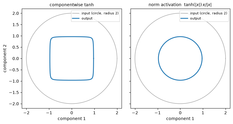
The input circle is mapped to itself by any rotation about its center, so an equivariant map must send it to another rotationally symmetric curve. The norm activation does (right: a smaller circle). Componentwise tanh instead produces a rounded square (left): it singles out the coordinate axes: the very axes equivariance says must be meaningless.

Norm activations are perfectly legitimate and appear in real architectures. However, Weiler et al. (2018) compared them against a third option and found it to “work in practice better” and to converge faster than tensor-product nonlinearities. That option is the gated nonlinearity, which is the standard nonlinearity of NequIP, MACE, and most of Part IV of this course.

7.3. The Gate

The gated nonlinearity was introduced by Weiler et al. in the 3D Steerable CNNs manuscript. For each non-scalar feature, \(f_i(x)\), the network produces one extra scalar field \(\gamma_i \star f(x)\) (in their voxel CNN: one more channel of the preceding convolution), squashes it with a sigmoid \(\sigma\), and rescales the feature by it. That is,

(5)\[ f_i(x) \;\longmapsto\; f_i(x)\, \sigma\big(\gamma_i \star f(x)\big). \]

The nonlinearity itself is parameter-free and manifestly equivariant: \(\sigma\) only ever acts on a scalar, and scalar \(\times\) feature is an allowed tensor-product path (\(0 \otimes l \to l\), Lesson 03a) that is realized channel-by-channel in e3nn through the ElementwiseTensorProduct as shown in Lesson 03b. Weiler et al. note that the gated nonlinearity can be read as a special case of both the norm nonlinearity (it changes only the length) and the tensor-product nonlinearity (one factor is a scalar).

The e3nn.nn.Gate enables this functionality together with ordinary activations for the scalar features. Its five constructor arguments describe an input split into three groups, \(x = (s, g, v)\) with irreps irreps_scalars + irreps_gates + irreps_gated:

argument	contents
irreps_scalars	scalars \(s\) that pass through their own activation (\(l = 0\) only)
act_scalars	the activation(s) applied to \(s\), one per entry of irreps_scalars
irreps_gates	scalars \(g\) consumed in gate: total multiplicity must match irreps_gated
act_gates	activation(s) for the gates, typically sigmoid
irreps_gated	the \(l > 0\) features \(v\) being gated

and computes (channel \(u\) of the gated block, gate scalar \(g_u\)):

(6)\[ \mathrm{Gate}(s, g, v) \;=\; \Big( \underbrace{\phi_s(s)}_{\text{activated scalars}},\; \underbrace{\phi_g(g_u)\, v_u}_{\text{gated features}} \Big), \qquad \mathtt{irreps\_out} = \mathtt{irreps\_scalars} + \mathtt{irreps\_gated}. \]

Note the bookkeeping: the gate scalars appear in irreps_in but not in irreps_out: they are consumed. The layer feeding a Gate must therefore produce those extra 0e channels (in Lesson 08, NequIP’s convolution does exactly this).

Let us see an example of a Gate in action.

# Create a Gate that takes 8 scalars, 4 gate scalars, and 2+2 non-scalar channels
gate = enn.Gate(
    "8x0e", [torch.nn.functional.silu],   # s: 8 scalars through SiLU
    "4x0e", [torch.sigmoid],              # g: 4 gate scalars through sigmoid ...
    "2x1o + 2x2e",                        # v: ... gating 2+2 = 4 non-scalar channels
)
print(gate)
print("irreps_in :", gate.irreps_in)
print("irreps_out:", gate.irreps_out, "  <- the 4x0e gates are consumed")
print(f"parameters: {sum(p.numel() for p in gate.parameters())}  (the Gate itself learns nothing)")
assert_equivariant(gate, gate.irreps_in, gate.irreps_out)

Gate (12x0e+2x1o+2x2e -> 8x0e+2x1o+2x2e)
irreps_in : 12x0e+2x1o+2x2e
irreps_out: 8x0e+2x1o+2x2e   <- the 4x0e gates are consumed
parameters: 0  (the Gate itself learns nothing)
equivariant!  (max error 8.882e-16 over random O(3) elements)

8.881784197001252e-16

7.3.1. The Gate, reproduced by hand

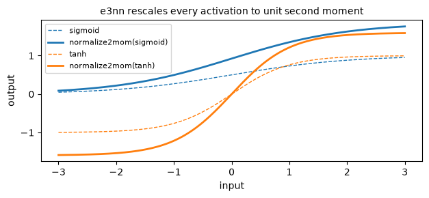
One subtlety before we replicate it: like all e3nn activations, the functions you pass in are silently wrapped with e3nn.math.normalize2mom, which rescales them by a fixed constant so that their output has unit second moment for standard-normal inputs. That is, \(\mathbb{E}_{z \sim \mathcal{N}(0,1)} [\varphi(z)^2] = 1\). This is the same variance bookkeeping as the path_weight constants of Lesson 03b. Note that every e3nn layer preserves unit variance in, unit variance out.

# The hidden rescaling inside every e3nn activation
from e3nn.math import normalize2mom

# Create a batch of 16 random inputs from the Gate, with the correct number of channels
x = gate.irreps_in.randn(16, -1)

# Scalars | gates | gated (2x1o: 6  +  2x2e: 10)
s, g, v = x.split([8, 4, 16], dim=-1)

# Reproduce the Gate by hand:  phi_s(s), phi_g(g) * v  per channel   (the gate equation)

# Activated scalars
phi_s = normalize2mom(torch.nn.functional.silu)(s)

# Activated gates
phi_g = normalize2mom(torch.sigmoid)(g)

# Gate u multiplies channel u
gated_1o = v[:, :6].reshape(16, 2, 3) * phi_g[:, 0:2, None]
gated_2e = v[:, 6:].reshape(16, 2, 5) * phi_g[:, 2:4, None]

# Concatenate the activated scalars and the gated features to form the manual output
manual = torch.cat([phi_s, gated_1o.reshape(16, 6), gated_2e.reshape(16, 10)], dim=-1)
print("Gate == ( phi_s(s), phi_g(g) * v ) :", torch.allclose(gate(x), manual))

Gate == ( phi_s(s), phi_g(g) * v ) : True

Let us now see how the normalize2mom wrapper impacts the sigmoid and tanh functions visually.

# Create a grid of input points for the activations
z = torch.linspace(-3, 3, 200)

# Visualize the effect of normalize2mom on the sigmoid and tanh functions
fig, ax = plt.subplots(figsize=(6.5, 3))
for f, name, c in [(torch.sigmoid, "sigmoid", "C0"), (torch.tanh, "tanh", "C1")]:
    ax.plot(z, f(z), color=c, ls="--", lw=1, label=name)
    ax.plot(z, normalize2mom(f)(z), color=c, lw=2, label=f"normalize2mom({name})")
ax.set_xlabel("input")
ax.set_ylabel("output")
ax.set_title("e3nn rescales every activation to unit second moment", fontsize=10)
ax.legend(fontsize=8)
fig.tight_layout()
plt.show()

7.4. The parity subtlety: even and odd scalars

The expression previously stated, “any function may act on a scalar”, was not entirely accurate. Under the \(O(3)\) group, there are two kinds of scalars (Lesson 02a): An even scalar, 0e, which has \(D(g) = 1\) for every \(g\): any \(\varphi\) is fine; and an odd scalar (pseudoscalar), 0o, which is invariant under rotations but flips sign under inversion: \(D(R) = 1\), \(D(P) = -1\). Equivariance of a pointwise \(\varphi\) on 0o requires that

(7)\[ \varphi(-x) = -\varphi(x) \qquad \rightarrow \qquad \varphi \text{ must be an odd function.} \]

As such, for example:

• \(\tanh\), \(\sin\), and \(x^3\) are odd functions. So, the output is again 0o.

• \(|x|\), \(\cos\), and \(x^2\) are even functions. Their usage is allowed, but the output becomes an even scalar, 0e, which means the sign information is destroyed as parities multiply: \(o \times o = e\).

• sigmoid, ReLU, SiLU are neither even nor odd functions. No output parity makes them equivariant. They break the \(O(3)\) symmetry.

Note that rotations never flip a pseudoscalar, so every test based on \(SO(3)\) operations passes and the bug is invisible until a reflected/inverted structure is used (recall Lesson 01a: chirality!). Our harness exposes it via its parity flag, which toggles whether random group elements include the inversion:

# The parity subtlety test
for act, name in [(torch.tanh, "tanh (odd)"), (torch.sigmoid, "sigmoid (neither)")]:
    
    # Rotations only
    err_so3 = equivariance_error(act, "0o", "0o", parity=False, n_trials=20)
    
    # Rotations + inversion
    err_o3 = equivariance_error(act, "0o", "0o", parity=True, n_trials=20)
    print(f"{name:22s} on 0o:   SO(3) error = {err_so3:.1e}    O(3) error = {err_o3:.1e}")

tanh (odd)             on 0o:   SO(3) error = 0.0e+00    O(3) error = 0.0e+00
sigmoid (neither)      on 0o:   SO(3) error = 0.0e+00    O(3) error = 1.0e+00

Sigmoid acting on a pseudoscalar is exactly \(SO(3)\)-equivariant and catastrophically wrong under \(O(3)\). The e3nn’s Activation (the module Gate uses internally for act_scalars/act_gates) refuses to let this happen: it probes your function’s parity at construction time and either tracks the output parity or raises an exception:

# E3nn refuses to let you apply a non-odd function to a pseudoscalar
try:
    enn.Activation("0o", [torch.sigmoid])
except ValueError as e:
    print("e3nn refuses:", e)

print("tanh on 0o ->", enn.Activation("0o", [torch.tanh]).irreps_out, "  (odd fn: parity kept)")
print("cos  on 0o ->", enn.Activation("0o", [torch.cos]).irreps_out, "  (even fn: parity flipped!)")

# The same algebra in the Gate: gating 1o features with 0o gates yields 1e outputs (o x o = e)
gate_odd = enn.Gate("0e", [torch.tanh], "4x0o", [torch.tanh], "4x1o")
print("odd gates:", gate_odd.irreps_in, "->", gate_odd.irreps_out)

# Check that it is equivariant
assert_equivariant(gate_odd, gate_odd.irreps_in, gate_odd.irreps_out)

e3nn refuses: Activation: the parity is violated! The input scalar is odd but the activation is neither even nor odd.
tanh on 0o -> 1x0o   (odd fn: parity kept)
cos  on 0o -> 1x0e   (even fn: parity flipped!)
odd gates: 4x0o+1x0e+4x1o -> 1x0e+4x1e
equivariant!  (max error 8.882e-16 over random O(3) elements)

8.881784197001252e-16

7.5. An equivariant MLP, end to end

We are now familiar with every ingredient of a full equivariant network: o3.Linear, the Gate, and an invariant readout via a tensor product. Let us assemble them and put the central promise of the course- “invariance by construction beats augmentation”- to a quantitative test.

7.5.1. Task

For a point cloud \(\{\vec r_1, \dots, \vec r_N\}\), predict the squared norm of its traceless second-moment (quadrupole) tensor, \(Q\), such that

(8)\[ X_i = \vec r_i - \bar{\vec r}, \qquad Q = \sum_{i=1}^N \Big( X_i X_i^\top - \tfrac{1}{3} |X_i|^2\, \mathbb{1} \Big), \qquad y = \| Q \|_F^2 . \]

Note that under \(g = (R, t)\) operations, we have \(X_i \to R X_i\), such that \(Q \to R Q R^\top\). Furthermore, this transformation leaves \(y\) unchanged because it is an \(E(3)\) invariant quantity (even under inversion, since \(Q\) is quadratic in \(X\)).

7.5.2. Equivariant embedding

The network needs a fixed-size equivariant description of the cloud. As in Lesson 02b, we embed directions with spherical harmonics, weight them by powers of the invariant radius, and sum over points (sums are permutation-invariant):

(9)\[ h^{(k)} = \frac{1}{\sqrt N} \sum_{i=1}^N |X_i|^k\; Y\big(\hat X_i\big), \qquad k \in \{1, 2\}, \qquad Y = \big(Y^{(0)}, Y^{(1)}, Y^{(2)}\big) . \]

Note that the hat denotes normalization to unit length, \(\hat X_i = X_i / |X_i|\), and \(Y^{(l)}\) are the spherical harmonics of degree \(l\) (Lesson 02b).

Each moment \(h^{(k)}\) carries irreps 0e + 1o + 2e (parities \((-1)^l\), Lesson 02b), so the full embedding \(h = (h^{(1)}, h^{(2)})\) has irreps_emb = 2 x (0e + 1o + 2e). This “sum of radially-weighted harmonics” is the core concept of the density trick behind ACE and MACE (Lesson 10). Note that the five components of \(Q\) are, up to a constant, exactly the \(l = 2\) part of \(h^{(2)}\): so, an exact solution exists inside our model class, but the network has to find (learn) it from the data.

7.5.3. Architecture

Two Linear \(\rightarrow\) Gate blocks, then an invariant readout that couples the hidden features with themselves into 0e (only \(l \otimes l \to 0\) paths survive: the readout is a learnable combination of invariant dot products):

(10)\[ h_1 = \mathrm{Gate}(W_1\, h), \qquad h_2 = \mathrm{Gate}(W_2\, h_1), \qquad \hat y = \big( h_2 \otimes_w h_2 \big)_{0e} . \]

7.5.4. Implementation

OK. Problem’s defined, architecture’s chosen, and the harness is ready. Let us get into the coding part. First, let us focus on creating the train/test dataset

# Seed the random number generator for reproducibility
torch.manual_seed(0)

# Points per cloud
N = 8

# Number of training and test clouds
B_train, B_test = 256, 128

# Create a tiny dataset of random clouds
pos_train = torch.randn(B_train, N, 3)    
pos_test = torch.randn(B_test, N, 3)

and the target function.

# Define the target function: the squared Frobenius norm of the traceless part
# of the second moment tensor of the point cloud
def target(pos):
    
    # Center the point cloud by subtracting the mean position
    X = pos - pos.mean(1, keepdim=True)
    
    # sum_i X_i X_i^T
    Q = torch.einsum("bni,bnj->bij", X, X)
    
    # Subtract the trace to make it traceless
    Q = Q - torch.eye(3) * Q.diagonal(dim1=1, dim2=2).sum(-1)[:, None, None] / 3
    
    # y = ||Q||_F^2
    return (Q**2).sum((1, 2))

Now, we calculate the labels for our dataset. We then calculate the mean and standard deviation of the labels and use them to standardize the labels. This is a common practice in machine learning to improve the convergence of the training process.

# Compute the target values for the training and test datasets
y_train, y_test = target(pos_train), target(pos_test)

# Compute the mean and standard deviation of the training labels
mu, sigma = y_train.mean(), y_train.std()

# Standardize the labels using the training statistics
y_train, y_test = (y_train - mu) / sigma, (y_test - mu) / sigma

# Create random rotation matrices for augmenting the test set
R = torch.stack([o3.rand_matrix() for _ in range(B_test)])

# The same test clouds in random orientations, never seen during training
pos_test_rot = torch.einsum("bij,bnj->bni", R, pos_test)
print("target is rotation-invariant, max |y(R pos) - y(pos)| =",
      f"{(target(pos_test_rot) - (y_test * sigma + mu)).abs().max().item():.2e}")

target is rotation-invariant, max |y(R pos) - y(pos)| = 1.14e-13

The dataset and target function are ready. The next step is to define the model architecture

# Seed the random number generator for reproducibility
torch.manual_seed(0)

# Spherical harmonic irreps: Y^(0), Y^(1), Y^(2)
sh_irreps = o3.Irreps("1x0e + 1x1o + 1x2e")

# Embedding irreps: two radial moments, k = 1 and k = 2
# Note: the l = 1 part of the k = 1 moment is sum_i r_i Y1(X_i-hat) = sum_i X_i, which
# centering forces to zero. Three of these 18 components are therefore structurally
# zero, and the 8 weights lin1 spends on that path never learn: the embedding really
# carries rank 15, not 18. Harmless here, but worth knowing when counting parameters.
irreps_emb = sh_irreps + sh_irreps

# Hidden irreps: 8 scalars, 8 vectors, 8 rank-2 tensors
irreps_hidden = o3.Irreps("8x0e + 8x1o + 8x2e")

# Define the equivariant MLP model
class EquivariantMLP(torch.nn.Module):
    def __init__(self):
        super().__init__()
        # Define the Gate that takes 8 scalars, 16 gate scalars, and 8+8 non-scalar channels
        make_gate = lambda: enn.Gate("8x0e", [torch.nn.functional.silu],   # Scalars
                                     "16x0e", [torch.sigmoid],             # 8+8 gate scalars
                                     "8x1o + 8x2e")                        # Gated features
        # Create two gates for the two hidden layers of the MLP
        self.gate1, self.gate2 = make_gate(), make_gate()
        # Produces the gates too!
        self.lin1 = o3.Linear(irreps_emb, self.gate1.irreps_in)
        self.lin2 = o3.Linear(irreps_hidden, self.gate2.irreps_in)
        # Readout layer: Fully connected tensor product to produce a scalar output
        self.readout = o3.FullyConnectedTensorProduct(irreps_hidden, irreps_hidden, "1x0e")

    # h^(k) = sum_i |X_i|^k Y(X_i-hat) / sqrt(N)
    def embed(self, pos):
        X = pos - pos.mean(-2, keepdim=True)
        r = X.norm(dim=-1, keepdim=True)
        Y = o3.spherical_harmonics([0, 1, 2], X, normalize=True, normalization="component")
        return torch.cat([(r * Y).sum(-2), (r**2 * Y).sum(-2)], dim=-1) / N**0.5

    def forward(self, pos):                          # pos: (B, N, 3) -> (B, 1)
        h = self.gate1(self.lin1(self.embed(pos)))   # h1 = Gate(W1 h)
        h = self.gate2(self.lin2(h))                 # h2 = Gate(W2 h1)
        return self.readout(h, h)                    # y-hat = (h2 (x) h2)_0e

# Create an instance of the EquivariantMLP model and print the number of parameters
model = EquivariantMLP()
print(f"Parameters: {sum(p.numel() for p in model.parameters())}")

Parameters: 592

Per course policy, we must test the equivariance BEFORE training. Here, the full E(3) pipeline is tested with random rotations x inversion x translations on raw positions

# Test on a batch of 8 point clouds
assert_model_equivariant(model, pos_test[:8], irreps_out="0e")

equivariant!  (max error 3.197e-14 over random O(3) + translations elements)

3.197442310920451e-14

7.5.5. Training with zero data augmentation

In Lesson 01a, we saw that a plain MLP on flattened coordinates only approximated invariance after heavy augmentation through rotation of the training data, with a worst-case invariance error some fourteen orders of magnitude above float64 round-off.

Here, we train on each point cloud in a single fixed orientation and evaluate on randomly rotated test clouds. The plain-MLP baseline below (same spirit as Lesson 01a’s model A, no augmentation) sees exactly the same data.

# Create a plain MLP that takes flattened coordinates as input and produces a scalar output
plain_mlp = torch.nn.Sequential(
    torch.nn.Linear(3 * N, 64), torch.nn.SiLU(),
    torch.nn.Linear(64, 64), torch.nn.SiLU(),
    torch.nn.Linear(64, 1),
)
print(f"plain MLP parameters: {sum(p.numel() for p in plain_mlp.parameters())}")

# Define a function to flatten and center the point cloud coordinates
def flatten_centered(pos):
    # Note that the plain MLP eats raw coordinates
    return (pos - pos.mean(1, keepdim=True)).reshape(len(pos), -1)

# Bookkeeping: store the networks and their corresponding feature extraction functions
nets = [("equivariant MLP", model, lambda p: p),
        ("plain MLP", plain_mlp, flatten_centered)]

# Train each network on the training data and record the losses
losses = {}
# Full-batch Adam, identical budgets
for name, net, feats in nets:
    opt = torch.optim.Adam(net.parameters(), lr=1e-2)
    losses[name] = []
    for step in range(1000):
        opt.zero_grad()
        loss = torch.nn.functional.mse_loss(net(feats(pos_train)).squeeze(-1), y_train)
        loss.backward()
        opt.step()
        losses[name].append(loss.item())
    print(f"{name:18s} final train MSE = {losses[name][-1]:.2e}")

plain MLP parameters: 5825
equivariant MLP    final train MSE = 9.38e-04
plain MLP          final train MSE = 2.74e-05

Let us now calculate the mean absolute error (MAE) for each network on the training set, test set, and rotated test set and comprare the results.

# Define a function to compute the mean absolute error (MAE) of a network on a
# given dataset
@torch.no_grad()
def mae(net, feats, pos, y):
    return (net(feats(pos)).squeeze(-1) - y).abs().mean().item()

# Compute the MAE for each network on the training set, test set, and rotated
# test set
results = {name: [mae(net, feats, pos_train, y_train),
                  mae(net, feats, pos_test, y_test),
                  mae(net, feats, pos_test_rot, y_test)] for name, net, feats in nets}

# Visualize the training losses and generalization errors for both networks
fig, axes = plt.subplots(1, 2, figsize=(9, 3.5))
colors = {"equivariant MLP": "C2", "plain MLP": "C0"}
for name in losses:
    axes[0].plot(losses[name], color=colors[name], label=name)
axes[0].set_yscale("log")
axes[0].set_xlabel("training step")
axes[0].set_ylabel("train MSE (standardized y)")
axes[0].set_title("training loss")
axes[0].legend(fontsize=8)

xpos = torch.arange(3)
for k, name in enumerate(results):
    axes[1].bar(xpos + 0.35 * k - 0.175, results[name], width=0.32,
                color=colors[name], label=name)
axes[1].set_xticks(xpos)
axes[1].set_xticklabels(["train", "test", "rotated test"])
axes[1].set_ylabel("MAE (standardized y)")
axes[1].set_title("generalization under rotation")
axes[1].legend(fontsize=8)
fig.tight_layout()
plt.show()

# Print the MAE results for each network
for name, (tr, te, rot) in results.items():
    print(f"{name:18s} MAE:  train {tr:.4f}   test {te:.4f}   rotated test {rot:.4f}")

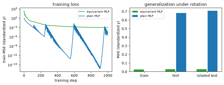
equivariant MLP    MAE:  train 0.0238   test 0.0262   rotated test 0.0262
plain MLP          MAE:  train 0.0009   test 0.6828   rotated test 0.7064

7.5.6. Analyzing the results

The plain MLP memorizes its 256 training point cloud data (train MAE \(\approx 0\)) but it does not effectively transfer that knowledge to either fresh clouds nor rotated ones in the testing sets: with \(3N = 24\) unconstrained inputs, this tiny dataset is hopeless. On the other hand, the equivariant MLP, with roughly 10× fewer parameters and zero data augmentation generalizes well and its rotated-test MAE equals its test MAE on the original test set to every printed digit. The invariance is not learned from the data, it is a property of the architecture, exactly as in Lesson 01a’s model C but now with a learnable, nonlinear network. This data-efficiency gap is the same phenomenon NequIP demonstrates on real molecules (Lesson 08).

7.6. Summary

In this lesson we learned:

• A pointwise nonlinear activation acting on the components of an \(l > 0\) irrep cannot be equivariant unless it becomes linear: rotations mix the feature components and \(\varphi\) acts on them one by one. We have verified these by observing \(O(1)\) error for tanh activation function acting on a 1x1o irrep feature.

• Legal nonlinearities can act on invariants: any \(\varphi\) can operate on 0e scalars. We introduced the norm activation, \(x \mapsto f(|x|)\, x / |x|\) (e3nn.nn.NormActivation), and reproduced its action from scratch.

• The Gate : extra 0e gate scalars, squashed and multiplied onto each \(l > 0\) channel by \(\big(\phi_s(s),\, \phi_g(g_u)\, v_u\big)\). The gate has zero parameters and does not learn anything: it is a nonlinearity that is manifestly equivariant. The e3nn package wraps all activations with a normalize2mom to ensure all outputs have unit second moment for standard-normal inputs.

• Parity: Odd 0o scalars admit only odd activations and even ones flip the output to 0e. The sigmoid function acting on 0o passes every \(SO(3)\) test yet breaks \(O(3)\): One should always test the equivariance with parity=True.

• A full equivariant MLP (o3.Linear \(\rightarrow\) Gate \(\rightarrow\) o3.Linear \(\rightarrow\) Gate \(\rightarrow\) tensor-product readout) trained on unrotated clouds generalizes to rotated test data with zero augmentation, at \(\approx\) 10x fewer parameters than a plain MLP, which fails to generalize.

Congratulations! You have come a long way and Part I is now complete. You are now familiar with symmetry types (Irreps), embeddings (spherical harmonics), linear/bilinear maps (tensor products), and nonlinearities (gates) which are essential for building equivariant neural networks.

Next: In Lesson 05a we move from from point clouds to graphs and discuss important concepts such as cutoff radii, neighbor lists, and periodic boundary conditions, the data structures many interatomic potentials are built on.

7.7. Exercises

Exercise 1: Parity bookkeeping (Difficulty: 🌶️): For each activation function, tanh, \(\sin\), \(x^2\), \(|x|\), sigmoid, acting on a single 0o scalar, decide: is it allowed, and what is the output parity? Verify each answer with enn.Activation("0o", [act]).

Solution

Odd functions keep 0o; even functions produce 0e; sigmoid is neither and e3nn must raise an exception for it.

# Check the parity of each activation function acting on a 0o scalar
for act, name in [(torch.tanh, "tanh"), (torch.sin, "sin"),
                  (lambda x: x**2, "x^2"), (torch.abs, "|x|"), (torch.sigmoid, "sigmoid")]:
    try:
        print(f"{name:8s} -> {enn.Activation('0o', [act]).irreps_out}")
    except ValueError:
        print(f"{name:8s} -> ValueError (neither even nor odd)")

# Output:
# tanh -> 1x0o, sin -> 1x0o, x^2 -> 1x0e, |x| -> 1x0e, sigmoid -> ValueError

Exercise 2: Norm activations instead of gates (Difficulty: 🌶️🌶️): Rebuild the MLP of Section 5 with each Gate replaced by enn.Activation on the 8x0e scalars plus enn.NormActivation on the 8x1o + 8x2e part (note: the Linears no longer need to produce gate scalars). Check equivariance and retrain. How does it compare?

Solution

class NormActMLP(torch.nn.Module):
    def __init__(self):
        super().__init__()
        # Linears produce only the scalars and gated features
        self.lin1 = o3.Linear(irreps_emb, irreps_hidden)
        self.lin2 = o3.Linear(irreps_hidden, irreps_hidden)
        # The scalars and gated features are activated separately
        self.act_s = enn.Activation("8x0e", [torch.nn.functional.silu])
        # NormActivation wants an Irreps object, not a string, when bias=True
        self.act_v = enn.NormActivation(o3.Irreps("8x1o + 8x2e"), torch.sigmoid, bias=True)
        # The readout is still a tensor product to 0e
        self.readout = o3.FullyConnectedTensorProduct(irreps_hidden, irreps_hidden, "1x0e")
        self.embed = model.embed # Reuse the embedding from the original model
    def act(self, h):
        return torch.cat([self.act_s(h[:, :8]), self.act_v(h[:, 8:])], dim=-1)

    def forward(self, pos):
        h = self.act(self.lin2(self.act(self.lin1(self.embed(pos)))))
        return self.readout(h, h)

# Instantiate the model and check equivariance on a small batch of test data
norm_model = NormActMLP()
assert_model_equivariant(norm_model, pos_test[:8], irreps_out="0e")

# ... then reuse the training loop.

At the same budget (1000 steps, lr 1e-2) this variant trains markedly worse: test MAE around 4x the gated model’s, and on some seeds it barely fits at all. That is not a capacity limit, given roughly 8x the steps it reaches a lower train MSE than the gated model. As NormActivation replaces each feature’s magnitude with \(\text{sigmoid}(||v|| + b)\) and discards the scale, the target (\(y = ||Q||_{F^2}\)) becomes scale-sensitive. This is the trainability gap Weiler et al. (2018) report, and why gates are the preferred choice for nonlinearity in practice (e.g., in NequIP and MACE).

Exercise 3: An equivariant output (Difficulty: 🌶️🌶️🌶️): Change the readout to o3.FullyConnectedTensorProduct(irreps_hidden, irreps_hidden, "1x1o") and train the network to predict the vector \(\vec p = \sum_i |X_i|^2 X_i\) (a 1o quantity: check its parity!). Verify with assert_model_equivariant(..., irreps_out="1o") that predictions co-rotate with the input.

Solution

The target property, \(\vec p\), is odd under inversion (\(X \to -X\) flips it) and rotates as a vector: irrep 1o. Note that \(\vec p = \sum_i r_i^3 \hat X_i\) is the \(l = 1\) part of the \(k = 3\) moment, while embed only builds \(k = 1\) and \(k = 2\): unlike the scalar target of Section 5, this one is not exactly representable from the embedding, so the training loss settles on a floor of roughly 1% of the target variance. Equivariance is exact either way, which is what this exercise checks.

# Define the target vector function
def target_vec(pos):
    X = pos - pos.mean(1, keepdim=True)
    # (B, 3), irreps 1o
    return ((X.norm(dim=-1, keepdim=True) ** 2) * X).sum(1)

# Instantiate the model
vec_model = EquivariantMLP()

# Inject the readout to produce a vector instead of a scalar. It stays a tensor
# product because forward() calls self.readout(h, h), with two arguments.
vec_model.readout = o3.FullyConnectedTensorProduct(irreps_hidden, irreps_hidden, "1x1o")

# Verify that the model is equivariant
assert_model_equivariant(vec_model, pos_test[:8], irreps_out="1o")

# Normalize the target vector for training
y_vec = target_vec(pos_train) / target_vec(pos_train).std()

# Define the optimizer
opt = torch.optim.Adam(vec_model.parameters(), lr=1e-2)

# Train the model for 600 steps
for step in range(600):
    opt.zero_grad()
    loss = torch.nn.functional.mse_loss(vec_model(pos_train), y_vec)
    loss.backward(); opt.step()
print(loss.item())   # settles near 0.01 -- the floor described above, not a bug

# ... and re-check equivariance after training!

7.8. References

• Geiger & Smidt, e3nn: Euclidean Neural Networks arXiv.2207.09453 (2021)

• Weiler et al., 3D Steerable CNNs NeurIPS (2018)

• Batzner et al., NequIP: E(3)-equivariant GNNs for interatomic potentials Nat. Commun. 13 2453 (2022)