14. Lesson 07c: The Rematch on Aspirin from rMD17

What you will learn

• Working with rMD17, one of the popular benchmark datasets: DFT energies and forces for organic molecules, its units, its official train/test splits. We also discuss the restrictions for using rMD17 which forbid training on more than 1000 of its frames.

• An apples-to-apples comparison of the same SchNet and SimpleDimeNet from Lessons 07a and 07b: same loss, optimizer, schedule and data budget with the only difference being the dataset.

• We perform an ablation study with angular basis truncated to a constant value to demonstrate that the gap in the prediction performance is caused by the angles themselves, not by the architecture differences.

• What triplets cost on a real molecule: from \(k \approx 4\) neighbors in our dilute argon gas to \(k \approx 15\) here: an order of magnitude more triplets per atom.

Prerequisites:

• Lesson 07a: SchNet, forces from autograd, the training pipeline,

• Lesson 07b: SimpleDimeNet, triplets, and the LJ-argon control experiment.

import sys
sys.path.insert(0, "..")    # Make course_utils importable

import copy, time, warnings
import numpy as np
import torch
import torch.nn as nn
import matplotlib.pyplot as plt
from e3nn import o3

from course_utils.data import load_rmd17, make_lj_argon_dataset, radius_graph
from course_utils.plotting import (plot_training_curves, scene3d,
                                    draw_point_cloud, show3d)
from course_utils.equivariance import assert_model_equivariant

warnings.filterwarnings("ignore", category=FutureWarning)  # ASE Langevin deprecation notice
torch.manual_seed(0)
np.random.seed(0)
device = "cuda" if torch.cuda.is_available() else "cpu"
silu = nn.functional.silu                    # swish, DimeNet's activation (see 07b)
print(f"device = {device}, torch {torch.__version__}")

device = cuda, torch 2.7.1+cu126

14.1. The rematch

Lesson 07b ended its training section with two notes. The first highlighted the fact that incorporating angular features into the model adds no missing physics for describing the Lennard-Jones potential in dilue argon gas system. Indeed the directional model (SimpleDimeNet) brought no advantage over SchNet (a distance-only model):

val MAE on LJ argon	E [meV/atom]	F [meV/Å]
SchNet	0.097	0.678
SimpleDimeNet	0.570	3.463

The second note suggested that for describing the physics of more realistic angle-dependent systems (e.g., molecules, covalent solids, the degenerate \(\mathcal{A}^\pm\) pairs) the picture changes dramatically. We will now proceed with training the same two models (SchNet and SimpleDimeNet) on the rMD17 dataset and see how the resulting performances change.

14.2. The rMD17 dataset

The revised MD17 rMD17 is a popular small-molecule benchmark dataset for training machine-learning potentials. It is a subset of the original MD17 dataset with the following properties:

• There are ten organic molecules, each with 100 000 structures taken from the original MD17 molecular-dynamics trajectories (Chmiela et al. 2017) at 500 K.

• The energies and forces are recomputed at the PBE/def2-SVP level with very tight SCF convergence and dense integration grids, making the labels practically free of numerical noise. (The original MD17 labels carry noise of roughly the size of the errors of a good model which is a serious problem when training models on forces.)

• Because the structures come from an MD trajectory, they are a correlated time series, not independent samples. The dataset’s own readme file states: “DO NOT train a model on more than 1000 samples from this dataset.” The authors provide official 1000-train/1000-test index splits. We use their split 01 and stay well below the cap.

• The units are kcal/mol and Å. Our loader function converts to the course units, eV and Å (1 kcal/mol = 43.36 meV).

Note: The course_utils.data.load_rmd17 module downloads the data artifacts once (\(\approx\) 150 MB), keeps the 2000 frames of the official split in a small (\(\approx\) 2 MB) local cache under artifacts/, deletes the big downloaded artifacts, and works offline afterwards.

Our molecule is aspirin, C\(_9\)H\(_8\)O\(_4\), 21 atoms which is objectively, the hardest case of the ten molecules with an aromatic ring, an ester and a carboxylic acid, connected by rotatable bonds. Thus, the system involves bends, torsions and conjugation in it, making its energy a function of angles. We proceed with the exact same data budget of Lessons 07a/07b: 150 training and 50 validation frames.

# Load the aspirin rMD17 dataset, and prepare the species map for the embeddings
train_frames, val_frames, z = load_rmd17("aspirin", n_train=150, n_val=50)

# Three elements in the data
# We map nuclear charge Z to a species index 0, 1, 2 for the embeddings
# {1:0, 6:1, 8:2}
species_map = {int(Z): s for s, Z in enumerate(torch.unique(z).tolist())}
species = torch.tensor([species_map[int(Z)] for Z in z])

# Count the number of species and atoms for later use
n_species, n_atoms = len(species_map), len(z)

# The common cutoff choice for the MD17 molecules (in Å)
R_CUT = 5.0

# Get the per-atom mean energy shift and the force standard deviation for the
# aspirin dataset
E_train = np.array([f["energy"] for f in train_frames])
eps_bar = E_train.mean() / n_atoms
F_std = torch.stack([f["forces"] for f in train_frames]).std()

# Print some statistics about the aspirin dataset
print(f"aspirin: {n_atoms} atoms, species map {species_map} (H, C, O)")
print(f"{len(train_frames)} train / {len(val_frames)} val frames (official rMD17 split 01)")
print(f"E fluctuations: std = {E_train.std()*1e3:.1f} meV  |  F std = {F_std*1e3:.1f} meV/Å")
print("compare LJ argon (07a):  E std =  21.3 meV  |  F std =   32.4 meV/Å")

aspirin: 21 atoms, species map {1: 0, 6: 1, 8: 2} (H, C, O)
150 train / 50 val frames (official rMD17 split 01)
E fluctuations: std = 269.4 meV  |  F std = 1273.3 meV/Å
compare LJ argon (07a):  E std =  21.3 meV  |  F std =   32.4 meV/Å

Comparing the force scale between aspirin and argon shows two very different worlds: The force components in aspirin have standard deviation of \(\approx\) 1.3 eV/Å instead of argon’s \(\approx\) 32 meV/Å. Covalent bonds are similar to stiff springs which produce large forces when stretched or compressed.

Note: The covalent skeleton (only bond-length pairs, \(d < 1.8\) Å), and the radius graph the models actually consume at \(r_\mathrm{cut} = 5\) Å. Aspirin’s diameter is only \(\approx\) 8 Å, so the model graph connects most pairs. So, the “dilute” regime of Lesson 07a does not exist here.

# Get the first training frame's positions
pos0 = train_frames[0]["pos"]

# Compute the radius graph for the covalent skeleton
# (bond-length pairs, d < 1.8 Å)
bonds = radius_graph(pos0, 1.8)

# Compute the radius graph for the model's cutoff
# (What SchNet / DimeNet actually see)
graph = radius_graph(pos0, R_CUT)

# Visualize the covalent skeleton and the model graph
fig = scene3d(1, 2, titles=[f"covalent skeleton ({bonds.shape[1]} directed edges)",
                            f"model graph, r_cut = {R_CUT} Å ({graph.shape[1]} directed edges)"],
              title_dy=-0.05)

# Draw the point cloud for the two graphs, coloring by element
elements = {1: ("H", "silver", 5), 6: ("C", "dimgray", 8), 8: ("O", "red", 8)}

for panel, edges in enumerate([bonds, graph]):
    draw_point_cloud(pos0, fig=fig, cell=(1, panel + 1), size=1, color="lightgray",
                     edges=edges)
    for Z_el, (name, color, size) in elements.items():
        draw_point_cloud(pos0[z == Z_el], fig=fig, cell=(1, panel + 1), color=color,
                         size=size, label=name if panel == 0 else None)
show3d(fig)

14.3. Changes between the rMD17 and argon datasets

14.3.1. The physics

Recall the classical force-field energy decomposition presented at the start of Lesson 07b:

(1)\[ E = E_\text{bonds} + E_\text{angle} + E_\text{torsion} + E_\text{non-bonding}. \]

For the LJ argon, only the last term exists. For aspirin, the angle and torsion terms are where the interesting chemistry happens. These are exactly the terms that the WL argument of Lesson 07b focuses on and states that a distance-based GNN cannot represent directly (it can only reconstruct them implicitly from patterns of overlapping distances, which demands additional data and depth).

14.3.2. The geometry

We use \(r_\mathrm{cut} = 5\) Å, which is a common choice for the MD17 molecules in the interatomic-potential literature. The cutoff radius is chosen to include all significant interactions while keeping the computational cost manageable. With this choice, the mean number of neighbors, \(k\), jumps by a factor of \(\approx\) 4 relative to our dilute argon gas and the triplet count, which scales as \(O(Nk^2)\) (Lesson 07b), by far more.

Let’s take one frame from the argon and aspirin subsets and count the number of neighbors and triplets, noting that

(2)\[ \#\text{triplets} = \sum_j \deg(j)\,(\deg(j) - 1) \]

# Get the positions of a single frame of LJ argon for comparison
argon_pos = make_lj_argon_dataset(n_frames=1)[0]["pos"]

# Print the table header
print(f"{'system':>17} | {'atoms':>5} | {'edges':>5} | {'k':>5} | {'triplets':>8} | {'trips/atom':>8}")

# Compute the radius graph and the number of triplets for both LJ argon and aspirin
for name, p, rc in [("LJ argon", argon_pos, 6.0), ("rMD17 aspirin", pos0, R_CUT)]:
    
    # Compute the radius graph for the given positions and cutoff
    ei = radius_graph(p, rc)
    
    # Neighbors within the cutoff
    deg = torch.bincount(ei[0], minlength=len(p))
    
    # sum_j deg(j)(deg(j)-1)
    n_trip = int((deg * (deg - 1)).sum())
    
    print(f"{name:>17} | {len(p):>5} | {ei.shape[1]:>5} | {ei.shape[1]/len(p):>5.1f} "
          f"| {n_trip:>8} | {n_trip/len(p):>10.1f}")

           system | atoms | edges |     k | triplets | trips/atom
         LJ argon |     8 |    30 |   3.8 |       96 |       12.0
    rMD17 aspirin |    21 |   294 |  14.0 |     4054 |      193.0

14.4. The contenders

Both SchNet and DimeNet models are re-implemented, word-by-word, from their home lessons: every line is derived and explained there (Lesson 07a for SchNet, Lesson07b for SimpleDimeNet). Here, they are just compressed into one cell each.

Before we proceed with training, note that:

• The species embedding represents more information: Lesson 07a used the nn.Embedding(n_species, F) module with a single species. In comparison, aspirin has three elements. Thus, the model uses n_species = 3 and the embedding now conveys more chemical information.

• The angular model is the smaller one: The SimpleDimeNet model has fewer parameters than the SchNet model. Specifically, the SimpleDimeNet model has approximately 51 k parameters, while the SchNet model has approximately 59 k parameters.

####################################
# SchNet (from Lesson 07a)
####################################

# Shifted softplus, ssp(0) = 0
def ssp(x):
    return nn.functional.softplus(x) - np.log(2.0)

class GaussianRBF(nn.Module):
    '''e_k(d) = exp(-gamma (d - mu_k)^2) on a regular grid of centers mu_k.'''
    
    def __init__(self, r_cut: float, n_rbf: int = 32, gamma: float = 10.0):
        super().__init__()
        self.register_buffer("mu", torch.linspace(0.0, r_cut, n_rbf))
        self.gamma = gamma
    
    # (E,) -> (E, n_rbf)
    def forward(self, d):
        return torch.exp(-self.gamma * (d.unsqueeze(-1) - self.mu) ** 2)

class FilterNet(nn.Module):
    '''W(d): RBF expansion -> two dense layers -> smooth cosine cutoff (Lesson 05b).'''
    
    def __init__(self, n_features: int, r_cut: float, n_rbf: int = 32):
        super().__init__()
        self.rbf = GaussianRBF(r_cut, n_rbf)
        self.dense1 = nn.Linear(n_rbf, n_features)
        self.dense2 = nn.Linear(n_features, n_features)
        self.r_cut = r_cut
    
    def forward(self, d):
        W = ssp(self.dense2(ssp(self.dense1(self.rbf(d)))))
        f_cut = 0.5 * (torch.cos(np.pi * d / self.r_cut) + 1.0)
        return W * f_cut.unsqueeze(-1)

class CFConv(nn.Module):
    '''Continuous-filter convolution:  x_i' = sum_{j in N(i)} x_j (*) W(d_ij).'''
    
    def __init__(self, n_features: int, r_cut: float):
        super().__init__()
        self.filter_net = FilterNet(n_features, r_cut)
        
    def forward(self, x, edge_index, d):
        # Receiver i, sender j (Lesson 05a)
        i, j = edge_index
        messages = x[j] * self.filter_net(d)
        return torch.zeros_like(x).index_add_(0, i, messages)

class InteractionBlock(nn.Module):
    '''x_i <- x_i + aw3( ssp( aw2( cfconv( aw1(x) ) ) ) )'''
    
    def __init__(self, n_features: int, r_cut: float):
        super().__init__()
        self.aw1 = nn.Linear(n_features, n_features)
        self.cfconv = CFConv(n_features, r_cut)
        self.aw2 = nn.Linear(n_features, n_features)
        self.aw3 = nn.Linear(n_features, n_features)
        
    def forward(self, x, edge_index, d):
        return x + self.aw3(ssp(self.aw2(self.cfconv(self.aw1(x), edge_index, d))))

class SchNet(nn.Module):
    '''Embedding -> T interaction blocks -> atom-wise readout, sum-pooled (07a).'''
    
    def __init__(self, n_features: int = 64, n_interactions: int = 3,
                 r_cut: float = 6.0, n_species: int = 1):
        super().__init__()
        self.embedding = nn.Embedding(n_species, n_features)
        self.interactions = nn.ModuleList(
            [InteractionBlock(n_features, r_cut) for _ in range(n_interactions)])
        self.readout1 = nn.Linear(n_features, n_features // 2)
        self.readout2 = nn.Linear(n_features // 2, 1)
        self.r_cut = r_cut
        
    def forward(self, pos, species, edge_index, batch, n_graphs):
        i, j = edge_index
        d = (pos[j] - pos[i]).norm(dim=-1)
        x = self.embedding(species)
        for block in self.interactions:
            x = block(x, edge_index, d)
        E_i = self.readout2(ssp(self.readout1(x))).squeeze(-1)
        E = torch.zeros(n_graphs, dtype=pos.dtype, device=pos.device)
        return E.index_add_(0, batch, E_i)

####################################
# SimpleDimeNet and its helpers
# (from Lesson 07b)
####################################

class BesselRBF(nn.Module):
    '''e_n(d) = u(d/c) sqrt(2/c) sin(n pi d / c) / d    (07b Eqs. (7) + (8), p = 6).'''
    
    def __init__(self, r_cut: float, n_rbf: int = 8, p: int = 6):
        super().__init__()
        self.register_buffer("n", torch.arange(1, n_rbf + 1, dtype=torch.get_default_dtype()))
        self.r_cut, self.p = r_cut, p
        
    def envelope(self, x):
        p = self.p
        return (1 - (p + 1) * (p + 2) / 2 * x**p + p * (p + 2) * x**(p + 1)
                - p * (p + 1) / 2 * x**(p + 2))
        
    def forward(self, d):
        x = (d / self.r_cut).unsqueeze(-1)
        e = np.sqrt(2.0 / self.r_cut) * torch.sin(self.n * np.pi * x) / d.unsqueeze(-1)
        return e * self.envelope(x)

def cos_basis(cos_alpha, n_ang: int):
    '''[1, cos a, cos 2a, ...] via the Chebyshev recursion (no arccos, see Lesson 07b).'''
    
    T = [torch.ones_like(cos_alpha), cos_alpha]
    for _ in range(n_ang - 2):
        T.append(2 * cos_alpha * T[-1] - T[-2])
    return torch.stack(T[:n_ang], dim=-1)

def find_triplets(edge_index):
    '''All edge pairs (a: k->j, b: j->i) with k != i, as indices into the edge list.'''
    
    recv, send = edge_index
    match = recv.unsqueeze(1) == send.unsqueeze(0)
    not_backtrack = send.unsqueeze(1) != recv.unsqueeze(0)
    a_idx, b_idx = (match & not_backtrack).nonzero(as_tuple=True)
    return a_idx, b_idx

class DirectionalInteraction(nn.Module):
    '''07b Eq. (4) with the DimeNet++-style Hadamard interaction.'''
    
    def __init__(self, F: int, n_rbf: int, n_ang: int):
        super().__init__()
        self.W_e = nn.Linear(n_rbf, F, bias=False)
        self.W_a = nn.Linear(n_rbf * n_ang, F, bias=False)
        self.W_m = nn.Linear(F, F)
        self.W_1 = nn.Linear(2 * F, F)
        self.W_2 = nn.Linear(F, F)
        
    def forward(self, m, e, a, trip_a, trip_b):
        t = self.W_e(e)[trip_b] * self.W_a(a) * silu(self.W_m(m[trip_a]))
        s = torch.zeros_like(m).index_add_(0, trip_b, t)
        return m + silu(self.W_2(silu(self.W_1(torch.cat([m, s], dim=-1)))))

class SimpleDimeNet(nn.Module):
    '''Directed-edge embeddings + directional message passing (Lesson07b, simplified).'''
    
    def __init__(self, n_features=64, n_blocks=2, r_cut=6.0, n_rbf=8, n_ang=6, n_species=1):
        super().__init__()
        self.rbf = BesselRBF(r_cut, n_rbf)
        self.embedding = nn.Embedding(n_species, n_features)
        self.edge_embed = nn.Linear(2 * n_features + n_rbf, n_features)
        self.blocks = nn.ModuleList(
            [DirectionalInteraction(n_features, n_rbf, n_ang) for _ in range(n_blocks)])
        self.readout1 = nn.Linear(n_features, n_features // 2)
        self.readout2 = nn.Linear(n_features // 2, 1)
        self.n_ang = n_ang
        
    def forward(self, pos, species, edge_index, trip_a, trip_b, batch, n_graphs):
        recv, send = edge_index
        d = (pos[send] - pos[recv]).norm(dim=-1)
        e = self.rbf(d)
        h = self.embedding(species)
        m = silu(self.edge_embed(torch.cat([h[send], h[recv], e], dim=-1)))
        # x_k - x_j
        u = pos[send[trip_a]] - pos[recv[trip_a]]
        # x_i - x_j
        v = pos[recv[trip_b]] - pos[send[trip_b]]
        cos_alpha = (u * v).sum(-1) / (u.norm(dim=-1) * v.norm(dim=-1))
        a = (self.rbf(u.norm(dim=-1)).unsqueeze(-1)
             * cos_basis(cos_alpha, self.n_ang).unsqueeze(-2)).flatten(-2)
        for block in self.blocks:
            m = block(m, e, a, trip_a, trip_b)
        # h_i = sum_j m_ji
        h_i = torch.zeros(len(pos), m.shape[-1], dtype=pos.dtype,
                          device=pos.device).index_add_(0, recv, m)
        E_i = self.readout2(silu(self.readout1(h_i))).squeeze(-1)
        E = torch.zeros(n_graphs, dtype=pos.dtype, device=pos.device)
        return E.index_add_(0, batch, E_i)

14.5. From full batch to mini-batches

One important change is necessary in the data preprocessing pipeline. The argon lessons trained the models on a full-batch of data: 150 frames of 8 atoms made a single graph of 1200 atoms and \(\approx\) 4000 edges. The same 150 frames of aspirin make \(\approx\) 45,000 edges and \(\approx\) 640,000 triplets, and training on forces backpropagates through the triplet tensor twice (create_graph=True).

This amount of data still fits on a GPU, but it is wasteful: one parameter update per epoch is a bad exchange rate for that much compute. We instead split the training set into mini-batches of 25 frames (six updates per epoch). The geometries are static, so all graphs and triplet lists are still precomputed once.

Again, we use the make_batch helper from Lesson 07b but with the species tensor now carrying real element indices.

# Set the batch size for training and validation
BATCH = 25

# Create mini-batches of training and validation data
def make_batch(frame_list, device):
    '''One disconnected graph: pos, species, edges, triplets, batch, E~, F  (as in 07b).'''
    
    pos, spec, edges, batch, E, F = [], [], [], [], [], []
    offset = 0
    for g, f in enumerate(frame_list):
        
        # Get the positions and append to the lists
        p = f["pos"].float()
        pos.append(p)
        
        # H/C/O indices, same for every frame
        spec.append(species)
        
        # Create the radius graph and append to the lists
        edges.append(radius_graph(p, R_CUT) + offset)
        
        # Create the batch index and append to the lists
        batch.append(torch.full((len(p),), g, dtype=torch.long))
        
        # Append the energy and forces to the lists
        E.append(f["energy"] - len(p) * eps_bar)
        F.append(f["forces"].float())
        
        # Update the offset for the next frame
        offset += len(p)
    
    # Concatenate the edges and find the triplets for the entire batch
    edge_index = torch.cat(edges, dim=1)
    # Precomputed once (static geometry)
    trip_a, trip_b = find_triplets(edge_index)
    
    # Return the concatenated tensors and move them to the specified device
    return (torch.cat(pos).to(device), torch.cat(spec).to(device),
            edge_index.to(device), trip_a.to(device), trip_b.to(device),
            torch.cat(batch).to(device),
            torch.tensor(E, dtype=torch.float32, device=device), torch.cat(F).to(device))

# Create mini-batches of training and validation data
train_batches = [make_batch(train_frames[i:i + BATCH], device)
                 for i in range(0, len(train_frames), BATCH)]
val_batch = make_batch(val_frames, device)

# Print the number of mini-batches, edges, and triplets in the training set
n_edges = sum(b[2].shape[1] for b in train_batches)
n_trips = sum(len(b[3]) for b in train_batches)
print(f"{len(train_batches)} mini-batches of {BATCH} frames | "
      f"train set total: {n_edges} edges, {n_trips} triplets "
      f"({n_trips / (len(train_frames) * n_atoms):.0f} per atom)")

6 mini-batches of 25 frames | train set total: 45402 edges, 642690 triplets (204 per atom)

14.6. Training protocol

We use the same training protocol for all models in this lesson. We adopt SchNet’s loss function with \(\rho = 1\), Adam optimizer with a learning rate of \(3\times10^{-3}\), cosine annealing, and train for 600 epochs. We compute forces using autograd: every knob is exactly the same as those in Lessons 07a and 07b and the only experimental variable is the dataset.

Two important notes:

• After the per-atom mean shift, aspirin’s energy fluctuations (\(\approx\) 13 meV/atom) are much smaller than its force components (\(\approx\) 1.3 eV/Å). As such, with \(\rho = 1\) the force term dominates the loss. That is standard practice for interatomic potentials as each frame carries \(3n = 63\) force labels against one energy label, and forces are what molecular dynamics consumes. Nonetheless, this means that the energy MAE rides along rather than being optimized hard.

• With a single fixed composition, the per-atom mean shift is just a constant offset. For datasets that mix molecules of different composition, the standard generalization is a least-squares fit of per-element reference energies. We will not, however, need it here.

Below, we implement one helper function (i.e., energy_and_forces) which routes each architecture’s inputs (SchNet consumes no triplets). So, a single training loop serves every model in this lesson:

# Helper functions to compute energy and forces based on the model
def energy_and_forces(model, batch, create_graph=False):
    '''E and F = -dE/dpos for either architecture (Lesson 07a).'''
    
    pos, spec, edge_index, trip_a, trip_b, bvec, E_ref, F_ref = batch
    pos = pos.requires_grad_(True)
    if isinstance(model, SimpleDimeNet):
        E = model(pos, spec, edge_index, trip_a, trip_b, bvec, len(E_ref))
    else:
        # SchNet: no triplets needed
        E = model(pos, spec, edge_index, bvec, len(E_ref))
    (dE_dpos,) = torch.autograd.grad(E.sum(), pos, create_graph=create_graph)
    return E, -dE_dpos

# Compute the mean absolute error (MAE) for energy and forces on a batch
def eval_mae(model, batch):
    '''(energy MAE [meV/atom], force MAE [meV/Å]) on one batch.'''
    
    E, F = energy_and_forces(model, batch)
    return ((E - batch[6]).abs().mean().item() / n_atoms * 1e3,
            (F - batch[7]).abs().mean().item() * 1e3)

# Compute the loss function for energy and forces, with optional weighting
def loss_fn(E, F, E_ref, F_ref, rho=1.0):
    return rho * ((E_ref - E) ** 2).mean() + ((F_ref - F) ** 2).sum(dim=-1).mean()

# Train the model for a specified number of epochs
def train(model, label, n_epochs=600, lr=3e-3):
    optimizer = torch.optim.Adam(model.parameters(), lr=lr)
    scheduler = torch.optim.lr_scheduler.CosineAnnealingLR(optimizer, T_max=n_epochs)
    history = {"train E MAE [meV/atom]": [], "val E MAE [meV/atom]": [],
               "train F MAE [meV/Å]": [], "val F MAE [meV/Å]": []}
    t0 = time.time()
    for epoch in range(n_epochs):
        model.train()
        for b in train_batches:
            optimizer.zero_grad()
            E, F = energy_and_forces(model, b, create_graph=True)
            loss_fn(E, F, b[6], b[7]).backward()
            optimizer.step()
        scheduler.step()
        tr = eval_mae(model, train_batches[0])           # first mini-batch as train proxy
        va = eval_mae(model, val_batch)
        for key, v in zip(history, (tr[0], va[0], tr[1], va[1])):
            history[key].append(v)
        if epoch % 100 == 0 or epoch == n_epochs - 1:
            print(f"[{label}] epoch {epoch:4d}   val E MAE {va[0]:7.3f} meV/atom   "
                  f"val F MAE {va[1]:8.2f} meV/Å")
    dt = time.time() - t0
    print(f"[{label}] training time: {dt:.0f} s on {device}")
    return history, dt

First, let’s train the distance-only model, SchNet. (Each of the three training cells in this lesson takes about a minute on an A100 GPU. Expect several minutes for each on CPU.)

# Set the random seed for reproducibility
torch.manual_seed(0)

# Initialize the SchNet model and print the number of parameters
schnet = SchNet(r_cut=R_CUT, n_species=n_species).to(device)
print("SchNet parameters:", sum(p.numel() for p in schnet.parameters()))

# Train the SchNet model and record the training history and time
hist_schnet, t_schnet = train(schnet, "SchNet")

SchNet parameters: 58561
[SchNet] epoch    0   val E MAE  20.866 meV/atom   val F MAE   934.93 meV/Å
[SchNet] epoch  100   val E MAE   7.784 meV/atom   val F MAE   225.97 meV/Å
[SchNet] epoch  200   val E MAE   3.139 meV/atom   val F MAE   181.00 meV/Å
[SchNet] epoch  300   val E MAE   2.849 meV/atom   val F MAE   154.51 meV/Å
[SchNet] epoch  400   val E MAE   2.586 meV/atom   val F MAE   137.39 meV/Å
[SchNet] epoch  500   val E MAE   2.740 meV/atom   val F MAE   130.72 meV/Å
[SchNet] epoch  599   val E MAE   2.362 meV/atom   val F MAE   129.51 meV/Å
[SchNet] training time: 66 s on cuda

It’s time to train our directional model, SimpleDimeNet on same data and with the same budget:

# Set the random seed for reproducibility
torch.manual_seed(0)

# Initialize the SimpleDimeNet model and print the number of parameters
dimenet = SimpleDimeNet(r_cut=R_CUT, n_species=n_species).to(device)
print("SimpleDimeNet parameters:", sum(p.numel() for p in dimenet.parameters()))

# Train the SimpleDimeNet model and record the training history and time
hist_dimenet, t_dimenet = train(dimenet, "SimpleDimeNet")

SimpleDimeNet parameters: 51393
[SimpleDimeNet] epoch    0   val E MAE 478.649 meV/atom   val F MAE   938.10 meV/Å
[SimpleDimeNet] epoch  100   val E MAE   4.554 meV/atom   val F MAE   162.93 meV/Å
[SimpleDimeNet] epoch  200   val E MAE   4.031 meV/atom   val F MAE   130.96 meV/Å
[SimpleDimeNet] epoch  300   val E MAE   2.264 meV/atom   val F MAE   110.70 meV/Å
[SimpleDimeNet] epoch  400   val E MAE   2.065 meV/atom   val F MAE   102.01 meV/Å
[SimpleDimeNet] epoch  500   val E MAE   2.091 meV/atom   val F MAE    98.30 meV/Å
[SimpleDimeNet] epoch  599   val E MAE   2.012 meV/atom   val F MAE    97.77 meV/Å
[SimpleDimeNet] training time: 81 s on cuda

14.7. Results

Let us now have the previous results on the argon dataset (from Lesson 07b) alongside the new aspirin results.:

# Set both models to evaluation mode
schnet.eval()
dimenet.eval()

# Evaluate the mean absolute error (MAE) for energy and forces on the validation
# batch for both models
e_s, f_s = eval_mae(schnet, val_batch)
e_d, f_d = eval_mae(dimenet, val_batch)

# Print the results on the aspirin dataset in a formatted table
print(f"{'val MAE':>22} | {'E [meV/atom]':>13} | {'F [meV/Å]':>10} | {'s/epoch':>8}")
print(f"{'SchNet (07a)':>22} | {e_s:>13.2f} | {f_s:>10.2f} | {t_schnet/600:>8.2f}")
print(f"{'SimpleDimeNet (07b)':>22} | {e_d:>13.2f} | {f_d:>10.2f} | {t_dimenet/600:>8.2f}")

# Print the force errors on both the LJ argon and aspirin datasets for comparison
print(f"\nforce MAE [meV/Å]{'':>6} | {'SchNet':>8} | {'SimpleDimeNet':>13}")
print(f"{'LJ argon (07b table)':>22} | {0.678:>8.3f} | {3.463:>13.3f}   <- distances suffice")
print(f"{'rMD17 aspirin':>22} | {f_s:>8.1f} | {f_d:>13.1f}   "
      f"<- angles matter ({f_s/f_d:.1f}x)")

               val MAE |  E [meV/atom] |  F [meV/Å] |  s/epoch
          SchNet (07a) |          2.36 |     129.51 |     0.11
   SimpleDimeNet (07b) |          2.01 |      97.77 |     0.13

force MAE [meV/Å]       |   SchNet | SimpleDimeNet
  LJ argon (07b table) |    0.678 |         3.463   <- distances suffice
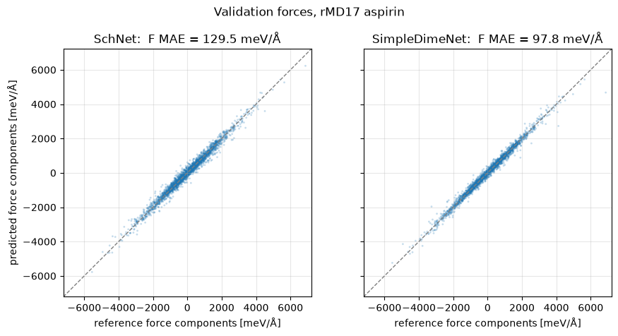
         rMD17 aspirin |    129.5 |          97.8   <- angles matter (1.3x)

# Plot the training curves for both models
ax = plot_training_curves({
    "SchNet val F MAE [meV/Å]": hist_schnet["val F MAE [meV/Å]"],
    "SimpleDimeNet val F MAE [meV/Å]": hist_dimenet["val F MAE [meV/Å]"],
    "SchNet train F MAE [meV/Å]": hist_schnet["train F MAE [meV/Å]"],
    "SimpleDimeNet train F MAE [meV/Å]": hist_dimenet["train F MAE [meV/Å]"],
})
ax.set_ylabel("force MAE [meV/Å]")
ax.set_title("rMD17 aspirin (150 frames): distance-only vs. directional")
ax.figure.tight_layout()

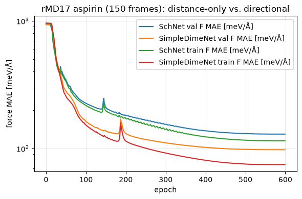
Looking at the training curves, we can see that the performance gap between the two models opens within the first hundred epochs. Each model’s training curve tracks its validation curve: the advantage shows up on unseen frames, not through memorization and overfitting.

Let us now look at the parity plots for forces using both models.

# Plot the predicted vs. reference forces for both models on the validation batch
F_true = val_batch[7].cpu().numpy().ravel() * 1e3

# Create a 1x2 subplot for the force comparison
fig, axes = plt.subplots(1, 2, figsize=(9.4, 4.6), sharex=True, sharey=True)
lim = np.abs(F_true).max() * 1.05
for ax, model, (label, f_mae) in zip(axes, [schnet, dimenet],
                                     [("SchNet", f_s), ("SimpleDimeNet", f_d)]):
    _, F_val = energy_and_forces(model, val_batch)
    F_pred = F_val.detach().cpu().numpy().ravel() * 1e3
    ax.plot([-lim, lim], [-lim, lim], "--", color="gray", lw=1)
    ax.scatter(F_true, F_pred, s=4, alpha=0.25, color="C0", edgecolors="none")
    ax.set_xlim(-lim, lim)
    ax.set_ylim(-lim, lim)
    ax.set_aspect("equal")
    ax.set_xlabel("reference force components [meV/Å]")
    ax.set_title(f"{label}:  F MAE = {f_mae:.1f} meV/Å")
    ax.grid(True, alpha=0.3)
axes[0].set_ylabel("predicted force components [meV/Å]")
fig.suptitle("Validation forces, rMD17 aspirin", y=1.0)
fig.tight_layout()

14.8. Is it really the angles?

The two architectures differ in more than just incorporating angles. They use different radial bases, edge instead of atom embeddings, and different activations. To pin down the gap due to the angles themselves, we run an ablation experiment from Lesson 07b’s Exercise 2 as a first-class case study here. To do so, we set n_ang = 1, so that the angular basis collapses to the constant \(T_0 = 1\). The resulting model still builds and pays for computing every triplet, still uses Bessel bases, edge embeddings and swish activation, but it just cannot resolve the angles between the edges.

# Set the random seed for reproducibility
torch.manual_seed(0)

# Initialize the angle-blind SimpleDimeNet model (n_ang=1) and print the number
# of parameters
dimenet_noang = SimpleDimeNet(r_cut=R_CUT, n_species=n_species, n_ang=1).to(device)
print("angle-blind SimpleDimeNet parameters:",
      sum(p.numel() for p in dimenet_noang.parameters()))

# Train the angle-blind SimpleDimeNet model and record the training history and
# time
hist_noang, t_noang = train(dimenet_noang, "SimpleDimeNet, n_ang=1")

angle-blind SimpleDimeNet parameters: 46273
[SimpleDimeNet, n_ang=1] epoch    0   val E MAE  71.136 meV/atom   val F MAE   936.37 meV/Å
[SimpleDimeNet, n_ang=1] epoch  100   val E MAE  10.074 meV/atom   val F MAE   271.18 meV/Å
[SimpleDimeNet, n_ang=1] epoch  200   val E MAE  12.068 meV/atom   val F MAE   214.66 meV/Å
[SimpleDimeNet, n_ang=1] epoch  300   val E MAE   4.643 meV/atom   val F MAE   186.17 meV/Å
[SimpleDimeNet, n_ang=1] epoch  400   val E MAE   4.071 meV/atom   val F MAE   173.46 meV/Å
[SimpleDimeNet, n_ang=1] epoch  500   val E MAE   7.565 meV/atom   val F MAE   168.16 meV/Å
[SimpleDimeNet, n_ang=1] epoch  599   val E MAE   3.866 meV/atom   val F MAE   167.43 meV/Å
[SimpleDimeNet, n_ang=1] training time: 65 s on cuda

After finishing the training, we can see how the angle-blind SimpleDimeNet model performs on the validation set

# Set the angle-blind SimpleDimeNet model to evaluation mode
dimenet_noang.eval()

# Evaluate the mean absolute error (MAE) for energy and forces on the validation
# batch for the angle-blind SimpleDimeNet model
e_n, f_n = eval_mae(dimenet_noang, val_batch)

# Print the results on the aspirin dataset in a formatted table, including the
# angle-blind SimpleDimeNet model
print(f"{'val MAE':>28} | {'E [meV/atom]':>13} | {'F [meV/Å]':>10}")
print(f"{'SchNet (Lesson 07a)':>28} | {e_s:>13.2f} | {f_s:>10.2f}")
print(f"{'SimpleDimeNet':>28} | {e_d:>13.2f} | {f_d:>10.2f}")
print(f"{'SimpleDimeNet, n_ang=1':>28} | {e_n:>13.2f} | {f_n:>10.2f}   <- angle-blind")

                     val MAE |  E [meV/atom] |  F [meV/Å]
         SchNet (Lesson 07a) |          2.36 |     129.51
               SimpleDimeNet |          2.01 |      97.77
      SimpleDimeNet, n_ang=1 |          3.87 |     167.43   <- angle-blind

14.9. Reading the result

• The reversal in the observed model performances is real: On the forces for the argon dataset, the directional model performed slightly worse than its distance-only counterpart (3.463 meV/Å for SimpleDimeNet vs. 0.678 meV/Å for SchNet). On the aspirin subset of the rMD17 dataset, SimpleDimeNet beats SchNet by a factor of \(\approx\) 1.3-1.5 in force MAE at an identical training budget and despite having fewer parameters.

  Note: The exact factor drifts a little between reruns (as GPU reductions are nondeterministic) but the ordering never does.

• The ablation study affirms our hypothesis on the importance of angular information: Blinding the SimpleDimeNet to angles turns its advantage into a deficit! The angle-blind variant is the worst of the three models studied here because it is just a clumsier distance-based model. The performance gap therefore lives in the angle-resolving basis functions \(T_m(\cos\alpha) = \cos(m\alpha)\) with \(m \geq 1\) that the ablation removed. Recall from Lesson 07b that the order \(m\) runs over \(0, \dots, n_\text{ang}-1\), and only the angle-independent \(m = 0\) term survives when n_ang = 1.

• The observed performance gap is smaller than the literature’s, and that is expected. Using 1000 training geometries, the full-size models are further apart on aspirin forces: 1.35 kcal/mol/Å (≈ 58.5 meV/Å) for SchNet vs. 0.499 kcal/mol/Å (≈ 21.6 meV/Å) for DimeNet (Gasteiger et al. 2020, MD17 benchmark). Our educational models are slimmer, our budget is 150 frames, and our separable radial \(\times\) cosine basis is weaker than the joint 2D basis. Note also that SchNet is far from helpless: message passing reconstructs a good deal of angular information implicitly (a neighbor’s distance pattern constrains angles), which is why the gap is a solid factor and not a collapse. The WL counterexample pairs \(\mathcal{A}^\pm\) of Lesson 07b are where implicit reconstruction provably fails, and real molecules sit in between.

• The triples impose a significant cost: For aspirin, we have \(\approx\) 200 triplets per atom instead of argon’s \(\approx\) 12. On a GPU, at 21 atoms, parallelism hides much of it (compare the s/epoch column above). On a CPU, or at liquid-density, The neighbor counts (\(k \approx 30\)-\(60\)), it does not: The Lesson 07b’s \(O(Nk^2)\) analysis is now a measured fact rather than a formula.

That last point is the cliffhanger for Part IV: The NequIP model carries directional information via its equivariant features (\(l > 0\)) on \(O(Nk)\) messages which translates into angular expressiveness without enumerating triplets.

14.10. Numerical verification of invariance

Similar to our previous equivariance checks in Lessons 07a and 07b, the energy must be a 0e scalar, and the forces 1o vectors. Here, we also cover the multi-species embedding path. The graph and triplets are rebuilt after each transform, so the whole pipeline is tested.

Recall that the course harness compares against e3nn’s D_from_matrix, which is itself only accurate to \(\sim 10^{-7}\) relative precision, and aspirin’s forces are \(\approx\) 40 \(\times\) larger than argon’s. As such, the harness’s absolute error floor rises accordingly (we allow \(10^{-5}\)). The direct check against \(R\) itself (for \(l = 1\) the Wigner \(D\) is the rotation matrix) confirms the exactness at float64 precision, as in Lesson 07b.

# Get a copy of the trained SimpleDimeNet model in double precision on the CPU
model64 = copy.deepcopy(dimenet).double().cpu().eval()

# Get the positions of the first validation frame and create a zero tensor for the
# batch index
pos_test = val_frames[0]["pos"].clone()
b_test = torch.zeros(n_atoms, dtype=torch.long)

# Define the energy function for the model, which computes the energy based on
# the positions and the radius graph
def energy_fn(pos):
    ei = radius_graph(pos.detach() if pos.requires_grad else pos, R_CUT)
    ta, tb = find_triplets(ei)
    return model64(pos, species, ei, ta, tb, b_test, 1).reshape(1)

# Define the force function for the model, which computes the forces as the
# negative gradient of the energy with respect to the positions
def force_fn(pos):
    pos = pos.requires_grad_(True)
    E = energy_fn(pos)
    (dE,) = torch.autograd.grad(E.sum(), pos)
    return -dE

# Check the equivariance of the energy and force functions under rotations and
# translations
print("energy  E(RX + t) = E(X):")
assert_model_equivariant(energy_fn, pos_test, "0e", tol=1e-12)
print("forces  F(RX + t) = R F(X)  (harness, tol limited by D_from_matrix ~1e-7 relative):")
assert_model_equivariant(force_fn, pos_test, "1o", tol=1e-5)

# Direct check against R (Lesson 07b)
err, F_ref = 0.0, force_fn(pos_test)
for _ in range(5):
    # Generate a random rotation matrix R
    R = o3.rand_matrix(dtype=torch.float64)
    
    # Improper rotations: parity too
    if torch.rand(()) < 0.5:
        R = -R
    
    # Generate a random translation vector t
    t = torch.randn(3, dtype=torch.float64)
    
    # Compute the maximum error between the transformed forces and the reference
    # forces
    err = max(err, (force_fn(pos_test @ R.T + t) - F_ref @ R.T).abs().max().item())

# Assert that the maximum error is below a specified tolerance and print the
# result
assert err < 1e-11, err
print(f"forces exactly covariant: max |F(RX+t) - R F(X)| = {err:.3e}  (float64)")

energy  E(RX + t) = E(X):
equivariant!  (max error 1.388e-15 over random O(3) + translations elements)
forces  F(RX + t) = R F(X)  (harness, tol limited by D_from_matrix ~1e-7 relative):
equivariant!  (max error 2.136e-06 over random O(3) + translations elements)
forces exactly covariant: max |F(RX+t) - R F(X)| = 5.507e-14  (float64)

14.11. Summary

In this lesson, we have learned:

• rMD17 provides high-quality DFT energies and forces for ten molecules, recomputed from the MD17 trajectories at the PBE/def2-SVP level of theory. Its frames are a correlated time series and the official splits involve training on no more than 1000 samples. Our data loader helper module caches the official split-01 frames locally and converts the units from kcal/mol to eV.

• The importance of angular information: We adopted the same SchNet and SimpleDimeNet models from Lessons 07a and 07b, and trained them with the same 150-frame training budget, same loss and optimizer, but with a different dataset (aspirin from rMD17 instead of argon). The results demostrated that when we train both models on molecules with bends, torsions and conjugation, such as aspirin, the directional message passing beats the distance-only model by \(\approx\) 1.3-1.5 \(\times\) on forces. The angle-blinded variant of SimpleDimeNet (n_ang=1) falls behind even SchNet, isolating the angles as the cause of the performance gap.

• Both baselines are now calibrated. Together, Lessons 07b and 07c show that investing in the architectural complexity pays off exactly when the data contains the corresponding physics in the target property that the model is trying to describe.

• The cost is real: Aspirin has \(k \approx 15\) neighbors and \(\approx\) 200 triplets per atom, an order of magnitude more triplets than argon. The \(O(Nk^2)\) triplet cost, predicted in Lesson 07b, is therefore no longer just a formula: it showed up as a measurable wall-clock penalty in the s/epoch column above.

Next: In Lesson 08a, we focus on the NequIP model which gains its angular (and higher) expressiveness from equivariant features at a \(O(Nk)\) cost in creating messages without incorporating triplets.

14.12. Exercises

1. Can depth substitute for angles? (Difficulty: 🌶️): Message passing lets a distance-only model reconstruct angular information implicitly, and more rounds mean more reconstruction. Retrain SchNet with n_interactions=6 (double the depth, \(\approx\) 115 k parameters, which is twice the SimpleDimeNet’s count). How much of the performance gap does depth close?

Solution

A deeper SchNet helps, but does not catch up with the directional model, SimpleDimeNet. In our runs, 6 interaction blocks improve SchNet’s force MAE only modestly (roughly 10-15 %). This still leaves a clear performance gap with respect to that of the directional model despite having twice as many parameters as SimpleDimeNet has. The implicit reconstruction of angular information in distance-only models requires a large amount of data: with only 150 frames the extra depth in SchNet mostly buys variance, not the missing representation. The fix is representational, not architectural scale: which is the whole thesis of Parts III-IV of this course.

2. A floppier, smaller molecule (Difficulty: 🌶️🌶️): Repeat the SchNet vs. SimpleDimeNet comparison on ethanol (load_rmd17("ethanol", ...): a \(\approx\) 67 MB one-time download that is cached as a 2 MB file). Use the same 150 train / 50 val frames, the same 600-epoch protocol, and the same performance score, i.e., the validation force MAE of each model and their ratio (the “performance gap”). Ethanol has only 9 atoms but two internal rotors: the hydroxyl (C-C-O-H) and methyl (H-C-C-O) torsions. So, its energy landscape is governed by dihedral angles.

Before running the experiment, make a prediction. Two effects will act in opposite directions: The torsional energetics involve the angular physics, which should favor the directional model. However, a 9-atom molecule has far fewer distinct atomic environments than a 21-atom one. So, 150 frames sample the ethanol’s configuration space much more densely and both models should find describing it easier. Do you expect the performance gap to be larger or smaller than the \(\approx\) 1.3 \(\times\) that we measured for aspirin? Check your prediction and report the results.

Solution

The helpers make_batch(), eval_mae() and train() read the molecule-specific variables (species, eps_bar, n_atoms, train_batches, val_batch) from the notebook namespace. So, switching molecules amounts to rebinding those variables and retraining. The code below does exactly that and prints the ethanol results next to the aspirin ones (f_s, f_d from the table above). Note that it overwrites the aspirin data variables: re-run the aspirin data cell to switch back.

# Load ethanol (C2H5OH): 9 atoms, the same three elements (H, C, O) as aspirin
train_frames, val_frames, z = load_rmd17("ethanol", n_train=150, n_val=50)

# Create the species tensor from the atomic numbers in z.
species_map = {int(Z): s for s, Z in enumerate(torch.unique(z).tolist())}
species = torch.tensor([species_map[int(Z)] for Z in z])

# Get the number of species and atoms
n_species, n_atoms = len(species_map), len(z)

# Compute the per-atom mean energy for the mean-shift
eps_bar = np.mean([f["energy"] for f in train_frames]) / n_atoms

# make_batch(), eval_mae() and train() read `species`, `eps_bar`, `n_atoms`,
# `train_batches` and `val_batch` from the notebook namespace, so rebinding them
# is all it takes to switch molecules (re-run the aspirin data cell to switch back)
train_batches = [make_batch(train_frames[i:i + BATCH], device)
                 for i in range(0, len(train_frames), BATCH)]
val_batch = make_batch(val_frames, device)

# Graph statistics: neighbors and triplets per atom (compare k ~ 15 and ~ 200 for aspirin)
n_frame_atoms = len(train_frames) * n_atoms
k_eth = sum(b[2].shape[1] for b in train_batches) / n_frame_atoms
trips_eth = sum(len(b[3]) for b in train_batches) / n_frame_atoms
print(f"ethanol: {n_atoms} atoms, k = {k_eth:.1f} neighbors, {trips_eth:.0f} triplets per atom\n")

# Train both models with the identical protocol used for aspirin
results = {}
for name, cls in [("SchNet", SchNet), ("SimpleDimeNet", SimpleDimeNet)]:
    torch.manual_seed(0)
    model = cls(r_cut=R_CUT, n_species=n_species).to(device)
    _, dt = train(model, f"{name} / ethanol")
    model.eval()
    results[name] = (*eval_mae(model, val_batch), dt / 600)

# Side-by-side with the aspirin results (f_s and f_d from the table above)
f_s_eth, f_d_eth = results["SchNet"][1], results["SimpleDimeNet"][1]
print(f"\n{'val force MAE [meV/Å]':>22} | {'SchNet':>8} | {'SimpleDimeNet':>13} | gap")
print(f"{'rMD17 aspirin':>22} | {f_s:>8.1f} | {f_d:>13.1f} | {f_s / f_d:.2f}x")
print(f"{'rMD17 ethanol':>22} | {f_s_eth:>8.1f} | {f_d_eth:>13.1f} | {f_s_eth / f_d_eth:.2f}x")
print(f"\nethanol s/epoch: SchNet {results['SchNet'][2]:.2f} | SimpleDimeNet {results['SimpleDimeNet'][2]:.2f}")

In our sample experiment, the two models reach 71.6 (SchNet) and 41.3 meV/Å (SimpleDimeNet) in validation force MAE. Thus:

• Both absolute errors drop by roughly half relative to aspirin (128.6 and 97.2 meV/Å): fewer atoms, fewer distinct environments, and the same 150 frames cover a 9-atom configuration space (in ethanol) much more densely than a 21-atom one (in aspirin).

• The performance gap widens from \(\approx\) 1.3 \(\times\) on aspirin to \(\approx\) 1.7 \(\times\) on ethanol. The directional model benefits most on the molecule whose energetics is dominated by torsions, described by dihedral angles. The exact performance gap ratios drift a little between reruns (GPU reductions are nondeterministic), but SimpleDimeNet stays clearly ahead.

• Bonus, the cost will be lower here, with \(k \approx 8\) neighbors, ethanol has \(\approx\) 56 triplets per atom instead of aspirin’s \(\approx\) 200, a \(\approx\) 4 \(\times\) reduction, exactly as the \(O(Nk^2)\) scaling of Lesson 07b predicts.

3. Sample efficiency (Difficulty: 🌶️🌶️🌶️): For \(n_\mathrm{train} \in \{50, 150, 450\}\) (all within the official 1000-frame split), train both models and plot validation force MAE against \(n_\mathrm{train}\) on a log–log scale. Which model extracts more from fewer frames, and why would an angular basis act as a “physics prior”?

Solution

Both curves fall roughly as a power law, with SimpleDimeNet’s sitting below SchNet’s at every budget (in our runs, \(\approx\) 55 vs. \(\approx\) 80 meV/Å at 450 frames). The angular basis hands the model \(\cos(m\alpha)\) features it would otherwise have to assemble indirectly from many correlated distance observations. Therefore, fewer samples are needed to constrain the angle-dependent part of the potential energy surface. Sample efficiency (not just final accuracy) is a recurring argument for building physics into the representation and we return to it in Part IV (NequIP’s headline result is reaching at similar accuracy from hundreds of frames).

14.13. References

• Chmiela et al., Machine learning of accurate energy-conserving molecular force fields Sci. Adv. 3 e1603015 (2017)

• Gasteiger et al., Directional Message Passing for Molecular Graphs arXiv.2003.03123 (2020)

• Schütt et al., SchNet: A continuous-filter convolutional neural network for modeling quantum interactions arXiv.1706.08566 (2017)