8. Lesson 05a: From Point Clouds to Atomistic Graphs

What you will learn

• Why atomistic machine learning represents a molecule or crystal as a graph where nodes correspond to atoms and edges to pairs of atoms closer than a cutoff radius, \(r_\mathrm{cut}\).

• The message-passing framework of graph neural networks (GNNs) and how atomistic models often adopt it.

• The course-wide edge convention, \(\vec{r}_{ij} = \vec{r}_j - \vec{r}_i\), (receiver \(i\), sender \(j\)) and why we often do not feed absolute positions to a network.

• How the cutoff radius controls graph connectivity and node degree.

• Periodic boundary conditions: minimum image, ASE neighbor lists, and why periodic edges need an extra edge_shift attribute.

Prerequisites:

• Lessons 01-04: Symmetry, irreps, tensor products, gates.

No e3nn is needed in this lesson: it is pure geometry and bookkeeping, but the conventions fixed here are used by every network in Parts II-V.

import sys
sys.path.insert(0, "..")    # Make course_utils importable

import matplotlib.pyplot as plt
import numpy as np
import torch
from e3nn import o3
from ase.build import molecule, bulk
from ase.neighborlist import neighbor_list

from course_utils.data import radius_graph
from course_utils.plotting import scene3d, draw_point_cloud, show3d

torch.manual_seed(0)
torch.set_default_dtype(torch.float64)  # Geometry lessons: exactness over speed
device = torch.device("cuda" if torch.cuda.is_available() else "cpu")
print(f"torch {torch.__version__} | device: {device}")

torch 2.7.1+cu126 | device: cuda

8.1. Why graphs? The local atomic environment picture

A configuration of matter can be modeled as a point cloud with attributes: a set \(\{(Z_i, \vec{r}_i)\}_{i=1}^N\) of atomic numbers and positions. Two physical facts shape how we process this information:

1. Locality. Chemical interactions are dominated by an atom’s near surroundings. This motivates the local atomic environment framework used by essentially all interatomic machine learning potentials. In this framework, the total energy is a sum of atomic contributions, where each term is a function of the atom’s neighborhood within some radius.

2. Symmetry. Properties are invariant/equivariant under permutations of identical atoms and under E(3) (Lessons 01-02). A set of atoms has no canonical ordering, so the architecture must be permutation-symmetric by construction.

Both properties are captured by the GNN architecture design. A GNN block updates the edge attributes, \(\mathbf{e}_k\) (edge \(k\) with receiver node \(r_k\) and sender node \(s_k\)), node attributes, \(\mathbf{v}_i\), and a global attribute, \(\mathbf{u}\), via three update functions, \(\phi\), and permutation-invariant aggregations \(\rho\):

(1)\[\begin{split} \begin{gather} \mathbf{e}'_k = \phi^e\!\left(\mathbf{e}_k, \mathbf{v}_{r_k}, \mathbf{v}_{s_k}, \mathbf{u}\right), \\ \mathbf{v}'_i = \phi^v\!\left(\bar{\mathbf{e}}'_i, \mathbf{v}_i, \mathbf{u}\right), \\ \bar{\mathbf{e}}'_i = \rho^{e\to v}\!\left(E'_i\right). \end{gather} \end{split}\]

Here, the atoms are representd by nodes, \(\mathbf{v}_i\), (and their attributes such as chemical species type, learned features \(h_i\), etc.), the nearby atomic pairs are connected through edges (alongside their edge attributes such as the relative vector \(\vec r_{ij}\), bond order, etc.), \(\phi^e\) denotes the message function, \(\phi^v\) is the node update function and \(\rho^{e \to v}\) is an aggregation function, often representinga sum over neighbors. Also, \(E'_i = \{(\mathbf{e}'_k, r_k, s_k)\}_{r_k = i}\) collects the updated edges arriving at node \(i\).

We should highlight that the specific choice of message function, node update function, and aggregation function can vary between different architectures. However, every architecture in this course, including SchNet, DimeNet, NequIP, and MACE, can be represented as a special GNN block iterated \(T\) times.

8.2. The radius graph and the edge convention

Given a set of position vectors, \(\{\vec{r}_i\}\), and a cutoff radius, \(r_\mathrm{cut}\), the radius graph has the directed edge set

(2)\[ \mathcal{E} \;=\; \bigl\{ (i, j) \;|\; i \neq j, \;\; \lVert \vec{r}_j - \vec{r}_i \rVert < r_\mathrm{cut} \bigr\}. \]

Each edge carries the relative (displacement) vector

(3)\[ \boxed{\;\vec{r}_{ij} \;=\; \vec{r}_j - \vec{r}_i\;} \qquad \text{($i$ = receiver, $j$ = sender: $\vec r_{ij}$ points from $i$ toward $j$).} \]

This sign/order convention is fixed for the whole course for consistency and convenience (see STYLE_GUIDE.md). In edge_index of shape (2, E), row 0 holds the receiver \(i\) and row 1 holds the sender \(j\): messages flow \(j \to i\). Since \(\lVert\vec r_{ij}\rVert = \lVert\vec r_{ji}\rVert\), the edge set is symmetric: both \((i,j)\) and \((j,i)\) are present, so the “directed” property of edges keeps the bookkeeping uniform while costs nothing extra.

Let us create our radius graph from a distance matrix, and a threshold value. We should be cautious to ensure the diagonal is removed so no atom becomes its own neighbor.

# Radius Graph
def radius_graph(pos, r_cut, loop=False):
    """Edge index (2, E): an edge (i <- j) whenever |r_j - r_i| < r_cut."""
    
    # (N, N) all pairwise distances
    dist = torch.cdist(pos, pos)
    
    # Boolean adjacency
    adj = dist < r_cut
    
    # Remove self-loops if requested
    if not loop:
        # An atom is not its own neighbor
        adj.fill_diagonal_(False)
        
    # Get the indices of the non-zero entries in the adjacency matrix
    receiver, sender = adj.nonzero(as_tuple=True)
    
    # row 0 = i, row 1 = j
    return torch.stack([receiver, sender])

Note: The brute-force algorithm will cost O(N²) which may be fine for the small systems in this course but production codes often use cell lists or k-d trees. This is exactly what course_utils.data.radius_graph implements and the later lessons import rather than redefine.

Let us see how we can calculate the edge indices for a simple organic molecule, ethanol (CH3CH2OH). We will use the ASE package to generate the atomic positions and then use our radius_graph function to compute the edges based on a cutoff radius.

# Ethanol: 2 C, 1 O, 6 H = 9 atoms
atoms = molecule("CH3CH2OH")

# Get the chemical symbols of the atoms
symbols = atoms.get_chemical_symbols()

# Get the Cartesian coordinates of the atoms
# (N, 3), Angstrom
pos = torch.tensor(atoms.get_positions())

# Angstrom
# Catches covalent bonds (C-H ~1.09, O-H ~0.97, C-C ~1.51, C-O ~1.43)
r_cut = 1.6

# (2, E)
edge_index = radius_graph(pos, r_cut)
print("atoms:", symbols)
print(f"N = {len(pos)} atoms, E = {edge_index.shape[1]} directed edges at r_cut = {r_cut} A")

atoms: ['C', 'C', 'O', 'H', 'H', 'H', 'H', 'H', 'H']
N = 9 atoms, E = 16 directed edges at r_cut = 1.6 A

With edge_index in hand, the per-edge geometry is two lines of indexing. Note carefully which row is which:

# i = receiver, j = sender
i, j = edge_index

# r_ij = r_j - r_i   <-> the boxed convention above
edge_vec = pos[j] - pos[i]

# |r_ij|
edge_len = edge_vec.norm(dim=-1)  

# Print the edges and their lengths
for k in range(0, 6):
    print(f"edge {symbols[j[k]]}(j={j[k]}) -> {symbols[i[k]]}(i={i[k]}):  |r_ij| = {edge_len[k]:.3f} A")

# Check that all edge lengths are in (0, r_cut)
assert (edge_len < r_cut).all() and (edge_len > 0).all()
print("all edge lengths in (0, r_cut) - as they must be")

edge C(j=1) -> C(i=0):  |r_ij| = 1.512 A
edge H(j=6) -> C(i=0):  |r_ij| = 1.093 A
edge H(j=7) -> C(i=0):  |r_ij| = 1.092 A
edge H(j=8) -> C(i=0):  |r_ij| = 1.092 A
edge C(j=0) -> C(i=1):  |r_ij| = 1.512 A
edge O(j=2) -> C(i=1):  |r_ij| = 1.427 A
all edge lengths in (0, r_cut) - as they must be

8.3. Translation invariance: why we do not use absolute positions as input

Under a global translation \(\vec r_i \mapsto \vec r_i + \vec t\), all absolute positions change, but every relative vector remains untouched:

(4)\[ \vec r_{ij} \;\mapsto\; (\vec r_j + \vec t) - (\vec r_i + \vec t) \;=\; \vec r_{ij}. \]

Under a rotation (or roto-inversion) \(g \in O(3)\), \(\vec r_i \mapsto g\,\vec r_i\), so \(\vec r_{ij} \mapsto g\, \vec r_{ij}\): the relative vector transforms as a clean \(l{=}1\) (vector) object with no inhomogeneous term. Furthermore, because \(\lVert g\,\vec r_{ij}\rVert = \lVert\vec r_{ij}\rVert\), the edge set itself is E(3)-invariant: symmetry operations never create or destroy edges.

A network fed only \(\{\vec r_{ij}\}\) (plus species) is therefore translation-invariant by construction: no data augmentation, no learning required on this part. However, feeding absolute positions would break this translation-invariance exactly (Lesson 01a: augmentation only ever approximates a symmetry the architecture doesn’t have). This is why every model in this course consumes edge vectors, never raw coordinates.

Let us analyze the effect of a global transformations of \(O(3)\) on the edge vectors and lengths for our ethanol molecule.

# Create a random translation vector
t = torch.randn(3)

# Create a random rotation matrix
R = o3.rand_matrix()

# Apply the translation and rotation to the positions
vec_translated = (pos + t)[j] - (pos + t)[i]
vec_rotated = (pos @ R.T)[j] - (pos @ R.T)[i]

print(f"translation:  max |r_ij(pos+t) - r_ij(pos)|      = {(vec_translated - edge_vec).abs().max():.2e}")
print(f"rotation:     max |r_ij(R pos)  - R r_ij(pos)|    = {(vec_rotated - edge_vec @ R.T).abs().max():.2e}")

# The edge set is invariant too: same distances => same graph
assert torch.equal(radius_graph(pos @ R.T + t, r_cut), edge_index)
print("edge_index(R pos + t) == edge_index(pos):  True")

translation:  max |r_ij(pos+t) - r_ij(pos)|      = 2.22e-16
rotation:     max |r_ij(R pos)  - R r_ij(pos)|    = 2.22e-16
edge_index(R pos + t) == edge_index(pos):  True

8.4. The cutoff radius controls the graph structure

The cutoff radius, \(r_\mathrm{cut}\), is one of the most important structural hyperparameter of an atomistic GNN:

• Too small of a \(r_\mathrm{cut}\) yields a disconnected graph over which the atoms can never exchange information (even with many message-passing layers).

• Too large of a \(r_\mathrm{cut}\) gives a graph with too many edges where the number of edges grows like \(N \cdot \langle \mathrm{deg}\rangle \propto N \, \rho \, r_\mathrm{cut}^3\) (density \(\rho\)), and with it memory and compute.

Typical interatomic potentials use \(r_\mathrm{cut} \approx 4\)–\(6\,\text{Å}\) which often covers a few coordination shells (we will see exact values for NequIP/MACE in Part IV). Note that message passing extends the effective receptive field to \(T \cdot r_\mathrm{cut}\) after \(T\) layers (Lesson 06a).

Let’s watch the ethanol graph fill in as we grow the cutoff:

# Create a list of cutoffs
cutoffs = [1.2, 1.6, 2.5, 4.0]

# Create a color map for the species
species_color = {"C": "dimgray", "O": "tab:red", "H": "lightskyblue"}
colors = [species_color[s] for s in symbols]

# Create a list of edge indices for each cutoff
eis = [radius_graph(pos, rc) for rc in cutoffs]

# Create a 1x4 scene with titles for each cutoff
fig = scene3d(1, 4, titles=[f"r_cut = {rc} A\n({ei.shape[1]} edges)"
                            for rc, ei in zip(cutoffs, eis)])
for a, ei in enumerate(eis):
    draw_point_cloud(pos, fig=fig, cell=(1, a + 1), color=colors, edges=ei)

# Show the figure
show3d(fig, title="Ethanol radius graph vs. cutoff (C gray, O red, H blue)", legend=False, title_dx=0.04)

At \(1.2\,\text{Å}\) only the X–H bonds appear (the heavy-atom skeleton is disconnected). At \(1.6\,\text{Å}\), we recover the chemical bond graph. By \(4\,\text{Å}\), the molecule is essentially a complete graph.

8.4.1. Degree statistics

The (in-)degree of the node \(i\) is defined as

(5)\[ \deg(i) = |\{j | (i,j) \in \mathcal{E}\}| \]

which is the number of neighbors it receives messages from. Its distribution vs. \(r_\mathrm{cut}\) can tell you the compute cost per atom and whether the graph is chemically meaningful:

# Calculate the number of atoms
N = len(pos)

# Create a figure with two subplots
fig, (axL, axR) = plt.subplots(1, 2, figsize=(11, 3.6))

# Left fig: mean degree as the cutoff sweeps
r_sweep = np.linspace(0.8, 5.0, 80)
mean_deg = [radius_graph(pos, rc).shape[1] / N for rc in r_sweep]
axL.plot(r_sweep, mean_deg)
axL.set_xlabel(r"$r_\mathrm{cut}$ [$\AA$]")
axL.set_ylabel("mean degree")
axL.set_title("mean node degree vs. cutoff")
axL.grid(alpha=0.3)

# Right fig: full degree histograms at the four cutoffs above
for rc in cutoffs:
    ei = radius_graph(pos, rc)
    # receivers -> in-degree
    deg = torch.bincount(ei[0], minlength=N)
    axR.hist(deg.numpy(), bins=np.arange(-0.5, N + 0.5), histtype="step",
             lw=2, label=rf"$r_\mathrm{{cut}}$={rc}")
axR.set_xlabel("node degree")
axR.set_ylabel("# atoms")
axR.set_title("degree histograms (ethanol, N=9)")
axR.legend()
axR.grid(alpha=0.3)
fig.tight_layout()
plt.show()

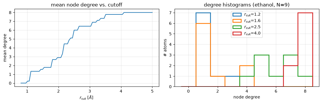
The mean degree is a staircase (edges switch on at each interatomic distance) that grows roughly like \(r_\mathrm{cut}^3\) once the environment looks homogeneous. For ethanol, it saturates at \(N-1 = 8\). This staircase is also a warning sign: quantities built from a hard cutoff can jump discontinuously as atoms move. This is the central problem of Lesson 05b.

8.5. Periodic boundary conditions

Crystals and liquids are simulated in a periodic cell: a matrix \(C \in \mathbb{R}^{3\times 3}\) whose rows \(\vec a_1, \vec a_2, \vec a_3\) are the lattice vectors. The real system contains atom \(j\) and all its periodic images

(6)\[ \vec r_j + \vec S \, C, \qquad \vec S = (n_1, n_2, n_3) \in \mathbb{Z}^3 . \]

An edge may therefore connect \(i\) to an image of \(j\), and its displacement vector needs the image offset:

(7)\[ \boxed{\;\vec r_{ij,\vec S} \;=\; \vec r_j + \vec S\, C - \vec r_i\;} \]

Two consequences that trip up every first implementation:

1. edge_index alone is ambiguous. The same pair \((i, j)\) can be connected through several images (different \(\vec S\)): even \(i = j\) (an atom bonds to its own image!). So a periodic graph must store the edge_shift, \(\vec S\), per edge, and the model must compute \(\vec r_{ij}\) from the formula above, never from pos[j] - pos[i].

2. Minimum image is not enough in general. The minimum-image convention keeps only the nearest image of each pair which is only valid when \(r_\mathrm{cut}\) is less than half the shortest cell height. ASE’s neighbor_list enumerates all images within \(r_\mathrm{cut}\), so it stays correct for small cells, where a cutoff sphere can wrap around the box and see the same atom several times.

A good example is a primitive fcc copper cell contains a single atom, yet every Cu atom has 12 nearest neighbors at \(a/\sqrt{2}\) all of which are images.

# Create a primitive cell with exactly ONE atom
cu = bulk("Cu", "fcc", a=3.6)
cell = torch.tensor(cu.cell.array)
print("Primitive fcc cell (rows = lattice vectors):\n", cell.numpy(), "\natoms in cell:", len(cu))

# Naive (non-periodic) graph: a single atom has no neighbors at all
print("Naive radius_graph edges:", radius_graph(torch.tensor(cu.positions), r_cut=2.6).shape[1])

# Periodic graph: ASE returns the receiver i, the sender j, and the image shift S
i_np, j_np, S_np = neighbor_list("ijS", cu, cutoff=2.6)
edge_index = torch.stack([torch.from_numpy(i_np).long(), torch.from_numpy(j_np).long()])
edge_shift = torch.from_numpy(S_np).to(torch.get_default_dtype())
i, j = edge_index

# Boxed formula: r_ij = r_j + S @ cell - r_i
edge_vec = cu.positions[j] + edge_shift.numpy() @ cell.numpy() - cu.positions[i]

# Compute the edge lengths
edge_len = np.linalg.norm(edge_vec, axis=-1)

print(f"Periodic edges: {edge_index.shape[1]}  (fcc coordination number = 12)")
print("All edges are self-edges (i=j=0), distinguished only by the shift S:")
print(edge_shift.to(torch.long).numpy().T)
print(f"Edge lengths: all = {edge_len.mean():.4f} A  (expected a/sqrt(2) = {3.6/np.sqrt(2):.4f} A)")
assert np.allclose(edge_len, 3.6 / np.sqrt(2))

Primitive fcc cell (rows = lattice vectors):
 [[0.  1.8 1.8]
 [1.8 0.  1.8]
 [1.8 1.8 0. ]] 
atoms in cell: 1
Naive radius_graph edges: 0
Periodic edges: 12  (fcc coordination number = 12)
All edges are self-edges (i=j=0), distinguished only by the shift S:
[[ 0  1  0  0  1 -1  1 -1  0  0 -1  0]
 [ 0  0  1 -1 -1  0  0  1  1 -1  0  0]
 [-1 -1 -1  0  0  0  0  0  0  1  1  1]]
Edge lengths: all = 2.5456 A  (expected a/sqrt(2) = 2.5456 A)

Every one of the 12 edges is \((i, j) = (0, 0)\) (print edge_index to verify!): without edge_shift they would be 12 copies of a zero-length self-loop and the model would see nothing. With the shifts, each edge acquires the correct displacement to a distinct neighboring image.

8.5.1. Cell-choice independence

Physics cannot depend on which repeating unit we draw. The conventional cubic fcc cell holds 4 atoms while the neighbor count per atom must still be 12:

# Create a conventional cubic cell: 4 atoms
cu4 = bulk("Cu", "fcc", a=3.6, cubic=True)

# Create the neighbor list
i4, j4, S4 = neighbor_list("ijS", cu4, cutoff=2.6)

# Create the edge index
ei4 = torch.stack([torch.from_numpy(i4).long(), torch.from_numpy(j4).long()])

# Create the edge shift tensor
shift4 = torch.from_numpy(S4).to(torch.get_default_dtype())

# Compute the degree of each atom
deg = torch.bincount(ei4[0], minlength=len(cu4))

# Count the number of edges that are within the home cell (S = 0)
n_zero = int((shift4 == 0).all(dim=1).sum())

print(f"Atoms: {len(cu4)}, edges: {ei4.shape[1]}, degree per atom: {deg.tolist()}")
print(f"Edges within the home cell (S = 0): {n_zero}, crossing the boundary (S != 0): {ei4.shape[1] - n_zero}")

Atoms: 4, edges: 48, degree per atom: [12, 12, 12, 12]
Edges within the home cell (S = 0): 12, crossing the boundary (S != 0): 36

Let’s visualize the central atom and its 12 image-neighbors reconstructed from \((j, S)\)

# Get the positions of the atoms in the conventional cell
center = torch.tensor(cu.positions[0])
neighbors = torch.tensor(cu.positions)[edge_index[1]] + edge_shift @ cell

# Atom 0 first, then its images, with a spoke drawn to each
shell = torch.cat([center[None, :], neighbors])
spokes = torch.stack([torch.zeros(len(neighbors), dtype=torch.long),
                      torch.arange(1, len(neighbors) + 1)])

# Create the 3D figure and draw the point cloud with edges
fig = scene3d()
draw_point_cloud(shell, fig=fig, edges=spokes,
                 color=["tab:red"] + ["tab:blue"] * len(neighbors))
show3d(fig, legend=False,
       title="fcc Cu: first coordination shell (red: atom 0), built from edge_shift")

8.6. Summary

In this lesson, we have learned:

• Atomistic ML often represents structures as radius graphs where nodes correspond to atoms and directed edges represent interactions (e.g., bonds) where \(\lVert\vec r_j - \vec r_i\rVert < r_\mathrm{cut}\).

• Convention (course-wide): The edge indices are stored in the edge_index object where the first row, edge_index[0], corresponds to the receiver \(i\), and the second row, edge_index[1], corresponds to the sender \(j\) Here, \(\vec r_{ij} = \vec r_j - \vec r_i\) and the messages flow from \(j \to i\).

• Relative vectors make translation invariance exact by construction. Rotations act on \(\vec r_{ij}\) as clean \(l{=}1\) vectors and leave the edge set invariant.

• The cutoff radius, \(r_\mathrm{cut}\), trades connectivity with computational cost (\(\langle\deg\rangle \propto r_\mathrm{cut}^3\)). The on/off switching of the edges causes the interaction discontinuity problem that Lesson 05b resolves.

• Periodic Boundary Condition (PBC): Under PBC, the edges connect to periodic images. Here, one stores the edge_shift tensor, \(\vec S\), and always compute \(\vec r_{ij} = \vec r_j + \vec S C - \vec r_i\) to get the correct displacement vector.

Next: Lesson 05b discusses the conversion of raw inter-node distances, \(|\vec r_{ij}|\), into well-behaved network feature inputs.

8.7. Exercises

1 (Difficulty: 🌶️): For ethanol, find the smallest cutoff (down to 0.1 Å) at which the radius graph remains connected (one component). Which bond sets the threshold?

Solution

import scipy.sparse as sp
import scipy.sparse.csgraph as csgraph

# Get the positions of the atoms in the conventional cell
for rc in np.arange(0.9, 2.0, 0.1):

    # Create the radius graph
    ei = radius_graph(pos, rc)

    # Convert to a sparse adjacency matrix and count connected components
    A = sp.coo_matrix((np.ones(ei.shape[1]), (ei[0], ei[1])), shape=(N, N))

    # Count the number of connected components
    n_comp, _ = csgraph.connected_components(A)

    # Print the results
    print(f"r_cut={rc:.1f}  components={n_comp}")

The graph becomes connected at \(r_\mathrm{cut} \geq 1.6\,\text{Å}\): the C–C bond (\(\approx 1.51\,\text{Å}\)) is the longest bond, so below it, the two carbon “islands” (each held together by shorter C–H / C–O / O–H bonds) stay separate.

2 (Difficulty: 🌶️🌶️): Implement the minimum-image displacement for an orthorhombic box (diagonal cell, lengths \(L_x, L_y, L_z\)). Writing the displacement in the course convention, \(\vec r_{ij} = \vec r_j - \vec r_i\), and letting \(\alpha \in \{x, y, z\}\) index its Cartesian components, each component wraps independently: \(r_{ij,\alpha} \mapsto r_{ij,\alpha} - L_\alpha \,\mathrm{round}(r_{ij,\alpha} / L_\alpha)\). Apply this formula to the conventional cubic Cu cell (cu4) with \(r_\mathrm{cut} = 1.7\,\text{Å} < L/2\) and check your code to see if it reproduces the neighbor_list edge lengths from ASE. Why must \(r_\mathrm{cut} < L/2\)?

Solution

# Create the pairwise displacement matrix and apply the minimum image convention
P = torch.tensor(cu4.positions)
L = torch.tensor(np.diag(cu4.cell.array))

# All pairwise r_j - r_i
d = P[None, :, :] - P[:, None, :]

# Apply the minimum image convention
d = d - L * torch.round(d / L)

# Calculate the pairwise distances and find edges within the cutoff
dist = d.norm(dim=-1).fill_diagonal_(np.inf)
ii, jj = (dist < 1.7).nonzero(as_tuple=True)

# Check that the distances match the neighbor_list output from ASE
i_ref, j_ref, S_ref = neighbor_list("ijS", cu4, 1.7)

# Reference edges
ei_ref = torch.stack([torch.from_numpy(i_ref).long(), torch.from_numpy(j_ref).long()])

# Reference shifts
sh_ref = torch.from_numpy(S_ref).to(torch.get_default_dtype())

# Make sure the edges match
assert len(ii) == ei_ref.shape[1]

The round function picks the single nearest image. If \(r_\mathrm{cut} \geq L/2\), an atom can be within the cutoff of two or more images of the same neighbor, but minimum image should only keep one edge. As such, it will silently drop the illigal interactions (here, \(L = 3.6\,\text{Å}\), so \(r_\mathrm{cut}=2.6\) would already be unsafe). That is why the neighbor_list function in ASE enumerates images instead.

3 (Difficulty: 🌶️🌶️): Assuming \(r_\mathrm{cut} = 5\,\text{Å}\), estimate the mean degree for fcc Cu (\(a=3.6\,\text{Å}\), 4 atoms per \(a^3\)). Verify your result with that of neighbor_list from ASE. Hint: Use the staircase plot of mean degree vs. cutoff radius. Analytically, for a homogeneous system of number density \(\rho\), one can write: \(\langle\deg\rangle = \tfrac{4}{3}\pi r_\mathrm{cut}^3 \rho\).

Solution

\(\rho = N/V = 4/3.6^3 = 0.0857\,\text{Å}^{-3}\),

So,

\(\langle\deg\rangle \approx \tfrac{4}{3}\pi \cdot (5)^3 \cdot 0.0857 \approx 44.9\).

Using ASE’s neighbor_list function, we can verify this estimate:

# Get the neighbor list for r_cut = 5.0 Å
i5, j5, _ = neighbor_list("ijS", cu, cutoff=5.0)

# Create the edge index tensor
ei = torch.stack([torch.from_numpy(i5).long(), torch.from_numpy(j5).long()])

# Calculate the mean degree
# 42 -- close; the discrete shells make it slightly lumpy
print(ei.shape[1] / len(cu))

8.8. References

• Battaglia et al., Relational inductive biases and graph networks arXiv.1806.01261 (2018)

• ASE documentation for ase.neighborlist.neighbor_list