6. Lesson 03b: Tensor Products in e3nn

What you will learn

• How e3nn generalizes the Clebsch–Gordan tensor product of Lesson 03a into a learnable layer: paths + per-path weights (\(x \otimes_w y\)).

• The anatomy of o3.TensorProduct: instructions, connection modes (uvw, uvu, …), path weights. Also, how to reproduce the output of o3.TensorProduct with a bare einsum.

• The convenience subclasses o3.FullyConnectedTensorProduct, o3.FullTensorProduct, o3.ElementwiseTensorProduct, and how to count their weights.

• Why a plain nn.Linear on raw irrep components breaks equivariance and why the “mix same-irrep channels only” special case does not.

Prerequisites:

• Lesson 02a: o3.Irreps

• Lesson 03a: Clebsch–Gordan decomposition, paths, Schur’s lemma

import sys
sys.path.insert(0, "..")    # Make course_utils importable

import torch
import matplotlib.pyplot as plt
from e3nn import o3

from course_utils.equivariance import assert_equivariant, equivariance_error

torch.set_default_dtype(torch.float64)   # Equivariance checks need double precision
torch.manual_seed(0)
device = "cuda" if torch.cuda.is_available() else "cpu"
print(f"torch {torch.__version__}, device = {device}")

torch 2.7.1+cu126, device = cuda

6.1. From CG paths to a learnable layer

Lesson 03a ended with Schur’s lemma: every equivariant bilinear map is a weighted sum of Clebsch–Gordan paths. e3nn turns that theorem into an engineering principle: a weighted tensor product \(x \otimes_w y\) whose free parameters are exactly one weight per path (or per channel combination within a path). This is the learnable layer of equivariant networks: in Tensor Field Networks, the convolution is a CG product of features with filters, and NequIP/MACE (Part IV) are built around the same weighted product.

Let \(x = (\vec x_1, \vec x_2)\) of type 1o + 1o and \(y = (y_1, \vec y_2)\) of type 0e + 1o. One can build an output of type 0e + 1o as shown below

(1)\[\begin{split} \begin{equation}(x, y) \mapsto z = \begin{pmatrix} w_1\, \vec x_1 \cdot \vec y_2 + w_2\, \vec x_2 \cdot \vec y_2 \\ w_3\, \vec x_1\, y_1 + w_4\, \vec x_2\, y_1 \end{pmatrix} \end{equation} \end{split}\]

Four paths, four weights \(w_1, \dots, w_4\): each path an allowed CG coupling (\(1 \otimes 1 \to 0\) dot products and \(1 \otimes 0 \to 1\) scalar–vector products). In e3nn:

# Creating a Fully Connected Tensor Product
tp = o3.FullyConnectedTensorProduct(
    irreps_in1="1o + 1o",       # x = (x1, x2), two vectors
    irreps_in2="0e + 1o",       # y = (y1, y2), a scalar and a vector
    irreps_out="0e + 1o",       # z = (z1, z2), a scalar and a vector
)

# Note: 4 paths | 4 weights, exactly w1..w4 of Eq. (1) in the notebook
print(tp)
print(f"Parameters: {sum(p.numel() for p in tp.parameters())}")

# Batch of 16 samples, each sample has 2 vectors or a scalar and a vector
x = o3.Irreps("1o + 1o").randn(16, -1)
y = o3.Irreps("0e + 1o").randn(16, -1)

# (16, 4): one 0e + one 1o
print("Output shape:", tuple(tp(x, y).shape))

FullyConnectedTensorProduct(2x1o x 1x0e+1x1o -> 1x0e+1x1o | 4 paths | 4 weights)
Parameters: 4
Output shape: (16, 4)

6.1.1. tp.instructions: the paths, spelled out

A TensorProduct is fully specified by its input/output Irreps plus a list of instructions. Each instruction is one path:

field	meaning
i_in1, i_in2, i_out	which entry of irreps_in1 / irreps_in2 / irreps_out the path connects (indices as irreps lists which must satisfy the selection rules, Eq. 5 of 03a)
connection_mode	how the channels (multiplicities) \(u, v, w\) of the three entries are wired
has_weight	whether the path carries learnable weights
path_weight	a fixed normalization constant (not learned) chosen so that each path contributes a unit variance
path_shape	the shape of this path’s weight block

# Print the details of each path in the tensor product
for ins in tp.instructions:
    ir1, ir2, ir3 = tp.irreps_in1[ins.i_in1].ir, tp.irreps_in2[ins.i_in2].ir, tp.irreps_out[ins.i_out].ir
    print(f"{ir1} (x) {ir2} -> {ir3}   {ins}")

1o (x) 0e -> 1o   Instruction(i_in1=0, i_in2=0, i_out=1, connection_mode='uvw', has_weight=True, path_weight=1.224744871391589, path_shape=(1, 1, 1))
1o (x) 1o -> 0e   Instruction(i_in1=0, i_in2=1, i_out=0, connection_mode='uvw', has_weight=True, path_weight=0.7071067811865476, path_shape=(1, 1, 1))
1o (x) 0e -> 1o   Instruction(i_in1=1, i_in2=0, i_out=1, connection_mode='uvw', has_weight=True, path_weight=1.224744871391589, path_shape=(1, 1, 1))
1o (x) 1o -> 0e   Instruction(i_in1=1, i_in2=1, i_out=0, connection_mode='uvw', has_weight=True, path_weight=0.7071067811865476, path_shape=(1, 1, 1))

e3nn offers a convenience method to visualize the paths in a diagram

# e3nn's built-in path diagram
fig, ax = tp.visualize()
fig.set_size_inches(5, 5)
plt.show()

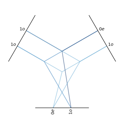
The diagram reads as the top-left the entries are from input 1, top-right from input 2, and the bottom from the outputs. Each curve through the center is one path/instruction.

6.2. Connection modes and the path equations

Within one path, the entries have multiplicities (channels): \(u = 1, \dots, m_1\) for input 1, \(v = 1, \dots, m_2\) for input 2, \(w\) for the output. The connection_mode says how they are wired. There are two main workhorses:

Fully connected (uvw): Every channel pair \((u, v)\) feeds every output channel \(w\), with an independent weight \(w_{uvw}\). So, the resulting path has \(m_1 m_2 m_3\) weights:

(2)\[ (\text{value of path})_{wk} = \frac{1}{\sqrt{m_1 m_2}} \sum_{u=1}^{m_1} \sum_{v=1}^{m_2} \sum_{i=1}^{2l_1+1} \sum_{j=1}^{2l_2+1} w_{uvw}\, C_{ijk}\, (\mathrm{in1})_{ui}\, (\mathrm{in2})_{vj} .\]

Input-1-preserving (uvu): The output inherits the channel index \(u\) of input 1 (\(m_3 = m_1\)), and only \((u, v)\) carries a weight (the \(m_1 m_2\) weights):

(3)\[ (\text{value of path})_{uk} = \frac{1}{\sqrt{m_2}} \sum_{v=1}^{m_2} \sum_{i=1}^{2l_1+1} \sum_{j=1}^{2l_2+1} w_{uv}\, C_{ijk}\, (\mathrm{in1})_{ui}\, (\mathrm{in2})_{vj} \]

Here, \(C_{ijk}\) denotes the CG coefficient, o3.wigner_3j(l1, l2, l3) and the prefactors, \(1/\sqrt{m_1 m_2}\) and \(1/\sqrt{m_2}\), keep the output variance at 1. When several paths land on the same output, the equations are additionally scaled by \(1/\sqrt{\#\text{paths}}\). All of these constants are folded into the path_weight parameter of the tensor product instructions. For details on other modes, (e.g., uuu, uvuv, …) see the e3nn documentation.

Let us build o3.TensorProduct from scratch using a single explicit instruction and reproduce its output only with wigner_3j and einsum to demistify its hidden complexities.

Terminology note: We call each instruction a path; e3nn’s printed repr instead counts the channel-resolved \((u, v, w)\) combinations, so one uvw instruction with \(m_1 m_2 m_3 = 6\) weights prints as “6 paths”. It is the object but with a finer-grained count.

First, we create a tensor product with one uvw instruction, connecting the first entry of input 1, the first entry of input 2, and the first entry of the output. The instruction carries weights, so the output is a learnable linear combination of the CG paths. We will check that the output of the tensor product is exactly the same as the explicit einsum of the CG coefficients with the input features and the weights.

# One 'uvw' path:  2x1o  (x)  1x1o  ->  3x0e 
# (a learnable, multi-channel dot product)
# (i_in1, i_in2, i_out, mode, has_weight)
tp_uvw = o3.TensorProduct(
    "2x1o", "1x1o", "3x0e",
    instructions=[(0, 0, 0, "uvw", True)],   
)
print(tp_uvw, "| weights:", tp_uvw.weight_numel, "= m1*m2*m3 = 2*1*3")

# 16 samples, 2 channels x 3 components
x = torch.randn(16, 6)
y = torch.randn(16, 3)

# Check the instructions of the tensor product
ins = tp_uvw.instructions[0]
print(f"Instruction: {ins} | weight shape: {tp_uvw.weight.shape} | path shape: {ins.path_shape}")

# (m1, m2, m3) = (2, 1, 3)
w = tp_uvw.weight.reshape(ins.path_shape)

# C.shape = (2l1+1=3, 2l2+1=3, 2l3+1=1)
C = o3.wigner_3j(1, 1, 0)

# Eq. (2), with the normalization constants folded into ins.path_weight:
manual = ins.path_weight * torch.einsum(
    "uvw,ijk,bui,bvj->bwk", w, C, x.reshape(16, 2, 3), y.reshape(16, 1, 3)
).reshape(16, 3)
print("einsum reproduces o3.TensorProduct ('uvw'):", torch.allclose(tp_uvw(x, y), manual))

TensorProduct(2x1o x 1x1o -> 3x0e | 6 paths | 6 weights) | weights: 6 = m1*m2*m3 = 2*1*3
Instruction: Instruction(i_in1=0, i_in2=0, i_out=0, connection_mode='uvw', has_weight=True, path_weight=0.7071067811865476, path_shape=(2, 1, 3)) | weight shape: torch.Size([6]) | path shape: (2, 1, 3)
einsum reproduces o3.TensorProduct ('uvw'): True

# same inputs, one 'uvu' path:  2x1o  (x)  1x1o  ->  2x1e
# (channel-wise cross products)
# (i_in1, i_in2, i_out, mode, has_weight)
tp_uvu = o3.TensorProduct(
    "2x1o", "1x1o", "2x1e",
    instructions=[(0, 0, 0, "uvu", True)],
)
print(tp_uvu, "| weights:", tp_uvu.weight_numel, "= m1*m2 = 2*1")

# Check the instructions of the tensor product
ins = tp_uvu.instructions[0]
print(f"Instruction: {ins} | weight shape: {tp_uvu.weight.shape} | path shape: {ins.path_shape}")

# (m1, m2) = (2, 1)
w = tp_uvu.weight.reshape(ins.path_shape)

# C.shape = (2l1+1=3, 2l2+1=3, 2l3+1=3)
C = o3.wigner_3j(1, 1, 1)

# Eq. (3): output keeps channel u
manual = ins.path_weight * torch.einsum(
    "uv,ijk,bui,bvj->buk", w, C, x.reshape(16, 2, 3), y.reshape(16, 1, 3)
).reshape(16, 6)
print("einsum reproduces o3.TensorProduct ('uvu'):", torch.allclose(tp_uvu(x, y), manual))

TensorProduct(2x1o x 1x1o -> 2x1e | 2 paths | 2 weights) | weights: 2 = m1*m2 = 2*1
Instruction: Instruction(i_in1=0, i_in2=0, i_out=0, connection_mode='uvu', has_weight=True, path_weight=1.7320508075688772, path_shape=(2, 1)) | weight shape: torch.Size([2]) | path shape: (2, 1)
einsum reproduces o3.TensorProduct ('uvu'): True

Both layers above are indeed one einsum with the CG tensor: everything else is bookkeeping. The uvw/uvu distinction matters at scale: uvw costs \(m_1 m_2 m_3\) weights per path (great capacity, expensive). On the other hand, uvu costs \(m_1 m_2\) (this is what NequIP uses in its convolutions, where input 2 is the spherical-harmonic edge embedding. We will discuss this topic in Lesson 08).

6.3. The convenience subclasses

6.3.1. o3.FullyConnectedTensorProduct

This function creates every selection-rule-allowed path with mode uvw. Its weight count is explicitly given by the formula

(4)\[ \#\text{weights} \;=\; \sum_{\substack{\text{allowed}\ (l_1, p_1),\, (l_2, p_2),\, (l_3, p_3)}} m_1\, m_2\, m_3 . \]

# A typical input feature layout
irreps1  = o3.Irreps("8x0e + 4x1o + 2x2e")

# E.g., spherical harmonics of an edge, l <= 2
irreps2  = o3.Irreps("1x0e + 1x1o + 1x2e")

# A typical output feature layout
irreps3  = o3.Irreps("8x0e + 4x1o + 2x2e")

# Fully connected tensor product: creates every selection-rule-allowed path with mode 'uvw'
fctp = o3.FullyConnectedTensorProduct(irreps1, irreps2, irreps3)
print(fctp)
print(f"parameters: {sum(p.numel() for p in fctp.parameters())}")

# Check the weight-count formula by explicit enumeration:
# (Selection rules)
n = sum(m1 * m2 * m3
        for m1, ir1 in irreps1 for m2, ir2 in irreps2 for m3, ir3 in irreps3
        if ir3 in ir1 * ir2)                    
print("formula gives:", n, "| e3nn says:", fctp.weight_numel)

FullyConnectedTensorProduct(8x0e+4x1o+2x2e x 1x0e+1x1o+1x2e -> 8x0e+4x1o+2x2e | 216 paths | 216 weights)
parameters: 216
formula gives: 216 | e3nn says: 216

# Cquivariance check (course policy): concatenate both inputs into one feature vector
def fctp_as_single_input(z):
    return fctp(z[:, : irreps1.dim], z[:, irreps1.dim :])

assert_equivariant(fctp_as_single_input, irreps_in=irreps1 + irreps2, irreps_out=irreps3)

equivariant!  (max error 3.242e-14 over random O(3) elements)

3.241851231905457e-14

6.3.2. o3.FullTensorProduct: The mathematician’s \(\otimes\)

Here, there are no weights or choices: all output irreps allowed by the selection rules are computed and kept. This is exactly the CG contraction we hand-built in Lesson 03a (e3nn scales each block by \(\sqrt{2 l_3 + 1}\) so that every output component has unit variance: the component normalization).

# 1o (x) 1o -> 0e + 1e + 2e, 0 weights
ftp = o3.FullTensorProduct("1o", "1o")
print(ftp)

# Create random input features for 16 samples, each with 3 components (1o)
xv, yv = torch.randn(16, 3), torch.randn(16, 3)

# Compute the manual CG contraction
manual = torch.cat(
    [(2 * l + 1) ** 0.5 * torch.einsum("ijk,bi,bj->bk", o3.wigner_3j(1, 1, l), xv, yv)
     for l in (0, 1, 2)], dim=-1)
print("FullTensorProduct == sqrt(2l3+1) * CG contraction of 03a:",
      torch.allclose(ftp(xv, yv), manual))

FullTensorProduct(1x1o x 1x1o -> 1x0e+1x1e+1x2e | 3 paths | 0 weights)
FullTensorProduct == sqrt(2l3+1) * CG contraction of 03a: True

6.3.3. o3.ElementwiseTensorProduct: Channel-aligned paths

In order to use this function, both inputs must have the same total multiplicity: channel \(u\) of input 1 is multiplied with channel \(u\) of input 2 (no mixing, no weights). This is the workhorse of gating (which we will discuss in Lesson 04) and of TFN-style products of features with per-channel filters.

# Channels are aligned in order: 0e*1o -> 1o,  0e*0e -> 0e,  1o*0e -> 1o
etp = o3.ElementwiseTensorProduct("2x0e + 1x1o", "1x1o + 2x0e")
print(etp)

# Define a function that wraps the ElementwiseTensorProduct to take a single input
def etp_as_single_input(z):
    return etp(z[:, : etp.irreps_in1.dim], z[:, etp.irreps_in1.dim :])

# Cquivariance check (course policy): concatenate both inputs into one feature vector
assert_equivariant(etp_as_single_input,
                   irreps_in=etp.irreps_in1 + etp.irreps_in2, irreps_out=etp.irreps_out)

ElementwiseTensorProduct(2x0e+1x1o x 1x1o+2x0e -> 1x1o+1x0e+1x1o | 3 paths | 0 weights)
equivariant!  (max error 8.882e-16 over random O(3) elements)

8.881784197001252e-16

The convinience functions at a glance:

class	paths	weights	typical use
o3.TensorProduct	you choose	you choose (uvw, uvu, …)	full control (NequIP, MACE internals)
o3.FullyConnectedTensorProduct	all allowed, uvw	\(\sum m_1 m_2 m_3\)	learnable mixing layer
o3.FullTensorProduct	all allowed	none	the mathematical \(\otimes\)
o3.ElementwiseTensorProduct	channel-aligned	none	gates, feature \(\times\) filter

6.4. What goes wrong without the machinery: a broken “linear layer”

Why insist on paths and CG coefficients even for something as simple as a linear layer? Because a dense matrix acting on the raw components of, say, a 0e + 1o feature freely mixes the scalar with individual vector components and a vector component alone is not an equivariant object. Let us demonstrate this with a simple example:

# 4 numbers: [s, vy, vz, vx]
irreps = o3.Irreps("0e + 1o")

# A plain dense 4x4 matrix
naive = torch.nn.Linear(irreps.dim, irreps.dim, bias=False)

# Check the equivariance error of the naive dense layer
err = equivariance_error(naive, irreps_in=irreps, irreps_out=irreps)
print(f"naive dense layer: max equivariance error = {err:.3f}   (should be ~1e-15 if equivariant)")

# Check the equivariance of the naive dense layer using assert_equivariant
try:
    assert_equivariant(naive, irreps_in=irreps, irreps_out=irreps)
except AssertionError as e:
    print("assert_equivariant:", e)

naive dense layer: max equivariance error = 2.954   (should be ~1e-15 if equivariant)
assert_equivariant: equivariance violated: max error 2.423e+00 >= tol 1.0e-09

The layer output changes depending on the orientation of the input. Any network containing such a layer loses every equivariance guarantees discussed in Lesson 01.

6.4.1. o3.Linear: The equivariant linear layer

Schur’s lemma (Lesson 03a, Sec. 6) tells us exactly which linear maps are allowed: within each irrep, channels may be mixed by arbitrary matrices \(W\) (the same \(W\) for all \(2l+1\) components \(m\)) and across different irreps, nothing mixes or interacts. The o3.Linear(irreps_in, irreps_out) function implements precisely this, so its weight count is \(\sum_{(l,p)} m_{\text{in}}^{(l,p)}\, m_{\text{out}}^{(l,p)}\) over matching irreps. It is the tensor product’s “unary” sibling and equivalent to a fully connected tensor product of the input with the constant scalar \(1\) (0e).

# Define an equivariant linear layer using o3.Linear
lin = o3.Linear("3x0e + 2x1o", "4x0e + 2x1o")

# 3*4 + 2*2 = 16 weights
print(lin)
print(f"parameters: {sum(p.numel() for p in lin.parameters())}")

# Check the equivariance of the o3.Linear layer using assert_equivariant
assert_equivariant(lin, irreps_in="3x0e + 2x1o", irreps_out="4x0e + 2x1o")

Linear(3x0e+2x1o -> 4x0e+2x1o | 16 weights)
parameters: 16
equivariant!  (max error 8.882e-16 over random O(3) elements)

8.881784197001252e-16

Now, let us visualize the outputs of a naive dense layer and an equivariant o3.Linear layer for a simple input.

# Visualize which outputs may depend on which inputs: the Jacobian of both layers
# The inputs are 4 numbers for the naive layer and 9 numbers for the o3.Linear layer
J_naive = torch.autograd.functional.jacobian(lambda z: naive(z), torch.randn(4))
J_lin = torch.autograd.functional.jacobian(lambda z: lin(z), torch.randn(9))

# The Jacobian matrices show the sensitivity of the outputs to the inputs.
# Plot the absolute values of the Jacobians to visualize which outputs depend on which inputs
fig, axes = plt.subplots(1, 2, figsize=(9, 4))
axes[0].imshow(J_naive.abs(), cmap="Greys")
axes[0].set_title("naive dense layer:\nevery component mixes (breaks equivariance)", fontsize=9)
axes[1].imshow(J_lin.abs(), cmap="Greys")
axes[1].set_title("o3.Linear 3x0e+2x1o -> 4x0e+2x1o:\nscalar block + per-m identity blocks", fontsize=9)
for ax in axes:
    ax.set_xlabel("input component")
    ax.set_ylabel("output component")
fig.tight_layout()
plt.show()

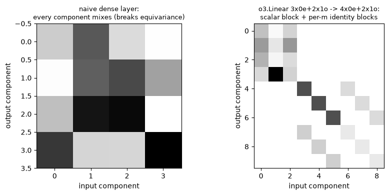
In the right panel, the top-left \(4 \times 3\) block mixes the scalar channels freely, while the vector part consists of \(2 \times 2\) channel mixing applied identically to each of the three \(m\) components (diagonal stripes): Schur’s lemma drawn as a picture: same irrep, same \(m\), mix channels only.

6.5. Summary

In this lesson, we learned that:

• e3nn’s o3.TensorProduct yields a list of CG paths (instructions), each optionally weighted: the complete parametrization of equivariant bilinear maps.

• The Connection modes wire the channels: The uvw mode demostrates a fully connected contraction with \(m_1 m_2 m_3\) weights per path (Eq. 2) vs. uvu with \(m_1 m_2\) weights whose output keeps the input-1’s channels, (Eq. 3). A fixed path_weight constant keeps the output variance at 1.

• We reproduced both contraction modes exactly with a single wigner_3j + einsum.

• The e3nn’s subclasses: FullyConnectedTensorProduct (all paths, learnable), FullTensorProduct (all paths, no weights = Lesson 03a’s \(\otimes\)), ElementwiseTensorProduct (channel-aligned, no weights: the gate’s engine).

• A plain dense layer operating on raw components of features fails the equivariance test with \(O(1)\) error. The o3.Linear (per-irrep channel mixing) is the equivariant replacement.

Next: Lesson 04 gives us the last missing ingredient: the equivariant nonlinearities (norm activations and the Gate), and our first full equivariant MLP.

6.6. Exercises

Exercise 1: count before you run (Difficulty: 🌶️🌶️): Without running it, compute the number of weights of o3.FullyConnectedTensorProduct("4x0e + 4x1o", "0e + 1o", "4x0e + 4x1o"). Then check.

Solution

Allowed \((ir_1, ir_2, ir_3)\) triples and their \(m_1 m_2 m_3\):

• \(0e{\times}0e{\to}0e\): \(4{\cdot}1{\cdot}4 = 16\)

• \(0e{\times}1o{\to}1o\): 16

• \(1o{\times}0e{\to}1o\): 16

• \(1o{\times}1o{\to}0e\): 16

• \(1o{\times}1o\to 1e, 2e\) are not in the output irreps

• Total 64

# Prints 64
print(o3.FullyConnectedTensorProduct("4x0e + 4x1o", "0e + 1o", "4x0e + 4x1o").weight_numel)

Exercise 2: The cross product as a TensorProduct (Difficulty: 🌶️): Build an unweighted o3.TensorProduct mapping 1x1o (x) 1x1o -> 1x1e with the single instruction (0, 0, 0, "uuu", False) (mode uvw requires weights; uuu works unweighted since all multiplicities are 1 here) and compare its output to torch.cross. What is the proportionality constant, and where does it come from? (Remember e3nn’s \((y, z, x)\) component order from Lesson 03a.)

Solution

# The unweighted tensor product computes the cross product up to a constant factor
tp_x = o3.TensorProduct("1o", "1o", "1e", [(0, 0, 0, "uuu", False)])

# Random vectors in R^3
a, b = torch.randn(3), torch.randn(3)

# Compute the tensor product
out = tp_x(a[None], b[None])[0]

# Reorder the components to match torch.cross's (x, y, z) order and compare
cart = [2, 0, 1]
print(out[cart] * 2**0.5, torch.cross(a[cart], b[cart], dim=0))

The constant is \(\sqrt 2\): the CG contraction gives \((\vec a \times \vec b)/\sqrt 6\) (Lesson 03a) and the component normalization multiplies by path_weight \(= \sqrt{2l_3+1} = \sqrt 3\), so e3nn returns \(\sqrt{3/6}\,(\vec a \times \vec b) = (\vec a \times \vec b)/\sqrt 2\).

Exercise 3: uvw vs. uvu at NequIP scale (Difficulty: 🌶️🌶️🌶️): For a convolution combining features 32x0e + 32x1o + 32x2e with edge harmonics 0e + 1o + 2e into 32x0e + 32x1o + 32x2e, how many weights are there for all-uvw paths (FullyConnectedTensorProduct) vs. the same paths in uvu mode? (For uvu, count \(m_1 m_2\) per allowed path.)

Solution

# Create the irreps
i1, i2, i3 = (o3.Irreps("32x0e + 32x1o + 32x2e"), o3.Irreps("0e + 1o + 2e"),
              o3.Irreps("32x0e + 32x1o + 32x2e"))

# Enumerate the allowed paths
paths = [(a, b, c) for a, (m1, ir1) in enumerate(i1) for b, (m2, ir2) in enumerate(i2)
         for c, (m3, ir3) in enumerate(i3) if ir3 in ir1 * ir2]

# Count the weights
# uvw: 11264
print(o3.FullyConnectedTensorProduct(i1, i2, i3).weight_numel)

# uvu: 352
tp_uvu = o3.TensorProduct(i1, i2, i3, [(a, b, c, "uvu", True) for a, b, c in paths])
print(tp_uvu.weight_numel)

There are 11 allowed paths. uvw: \(11 \times 32 \cdot 1 \cdot 32 = 11264\). uvu: \(11 \times 32 \cdot 1 = 352\): a factor \(m_3 = 32\) fewer. This economy is why NequIP-style convolutions use uvu and delegate channel mixing to separate o3.Linear layers.

6.7. References

• Geiger & Smidt, e3nn: Euclidean Neural Networks arXiv.2207.09453 (2021)

• Thomas et al., Tensor Field Networks arXiv.1802.08219 (2018)