11. Lesson 06b: The Tetris Example

What you will learn

• Batching several small graphs into one by using the index-offset trick

• Why a model, whose output contains only true scalars (0e), cannot distinguish mirror-image shapes in the 3D Tetris dataset, and how using a pseudoscalar (0o) output fixes this issue

• The augmentation-free rotation test: train on one orientation, evaluate on random rotations

• Bonus: Inverting the shapes swaps the chiral pair’s predictions due to equivariance acting on labels.

Prerequisites:

• Lesson 02a: Parity

• Lessons 04, 05a, and 05b: gates,

• Lesson 06a: The TFNConv block,

import sys
sys.path.insert(0, "..")    # Make course_utils importable

import math

import matplotlib.pyplot as plt
import numpy as np
import torch
from e3nn import o3, nn as enn

from course_utils.data import radius_graph, tetris, TETRIS_LABELS
from course_utils.equivariance import assert_model_equivariant
from course_utils.plotting import (scene3d, draw_point_cloud, show3d,
                                    plot_training_curves)

torch.manual_seed(0)
torch.set_default_dtype(torch.float64)  # Tiny model: keep the precision, verify equivariance
device = torch.device("cpu")            # 32 atoms total - CPU is instant
print(f"torch {torch.__version__}")

torch 2.7.1+cu126

11.1. The 3D Tetris dataset: Eight shapes, one chiral pair

The 3D Tetris dataset offers a classic e3nn exercise where the an equivariant model is tasked to classify eight 3D “Tetris” shapes. The course provides a convenience function to create the Tetris dataset: course_utils.data.tetris() returns eight shapes, each made out of four unit blocks, representing a point cloud of 4 atoms per shape. Shapes 0 and 1, chiral_shape_1 and chiral_shape_2, are mirror images of each other: no rotation or translation maps one onto the other, only an improper operation (reflection/inversion) does.

Note: Any network that relies solely upon distances (such as SchNet) or angles between points (such as ANI-1) cannot distinguish the chiral shapes from each other but equivariant models such as tensor field networks (TFNs) can.

Note: The tetris() coordinates are copied row-for-row from the reference code’s shape_classification.ipynb; only three names differ — the repo’s T/zigzag/L labels are our L/T/zigzag (we keep the e3nn tutorial’s naming, which matches the geometry).

We should also point out that the TFN is formulated for SO(3) (rotations only). Thus, chirality-sensitivity comes for free in its \(l=0\) outputs. e3nn works with the full O(3) and tracks parity explicitly (Lesson 02a). So, chirality-sensitivity must be declared, by giving the output a pseudoscalar 0o slot. That distinction is the whole point of this lesson.

Let us look at the shapes in the 3D Tetris dataset.

# Load the 3D Tetris dataset
# (8, 4, 3), (8, 8)
pos8, labels_onehot = tetris()
print("shapes:", TETRIS_LABELS)

# Visualize the 8 Tetris shapes
# Unit blocks: catches side (1.0) + diagonal (sqrt 2) pairs
r_cut = 1.5

# Chirality is the whole point here, and it only reads properly in 3D
fig = scene3d(2, 4, titles=[f"{k}: {TETRIS_LABELS[k]}" for k in range(len(pos8))])

for k, p in enumerate(pos8):
    draw_point_cloud(p, fig=fig, cell=(k // 4 + 1, k % 4 + 1),
                     color="tab:red" if k < 2 else "C0", edges=radius_graph(p, r_cut))

show3d(fig, title="the 8 Tetris shapes (red: the chiral mirror pair)", legend=False)

shapes: ['chiral_shape_1', 'chiral_shape_2', 'square', 'line', 'corner', 'L', 'T', 'zigzag']

11.2. Batching the eight graphs

The whole dataset fits in one forward pass if we concatenate the graphs. The node indices of shape \(g\) are offset by the number of preceding nodes, and a batch vector remembers which graph each node belongs to. Thus, we can pool node features per graph at the end (mean over each shape’s 4 blocks, which is a linear and permutation-invariant operation) making the readout also equivariant. Note that the global pooling operation, mentioned here, is equivariant because D-matrices act linearly.

Let us see how to implement this batching trick.

# Batching the eight graphs
def batch_graphs(pos_list, r_cut):
    
    # Containers for positions, edges, and batch vectors
    positions, edges, batch, offset = [], [], [], 0
    
    # Iterate over each graph in the list
    for g, p in enumerate(pos_list):
        
        # Append the positions, edges, and batch vector for the current graph
        positions.append(p)
        edges.append(radius_graph(p, r_cut) + offset)
        batch.append(torch.full((len(p),), g, dtype=torch.long))
        
        # Update the offset for the next graph
        offset += len(p)
        
    # Concatenate the positions, edges, and batch vectors into single tensors
    return torch.cat(positions), torch.cat(edges, dim=1), torch.cat(batch)

# Batch the graphs and print the number of nodes, edges, and average degree
pos, edge_index, batch = batch_graphs(list(pos8), r_cut)
avg_neighbors = edge_index.shape[1] / len(pos)

# Print the number of nodes, edges, and average degree of the batched graph
print(f"batched: {len(pos)} nodes, {edge_index.shape[1]} edges, <deg> = {avg_neighbors:.2f}")
print(f"batch vector: {batch.tolist()}")

batched: 32 nodes, 78 edges, <deg> = 2.44
batch vector: [0, 0, 0, 0, 1, 1, 1, 1, 2, 2, 2, 2, 3, 3, 3, 3, 4, 4, 4, 4, 5, 5, 5, 5, 6, 6, 6, 6, 7, 7, 7, 7]

11.3. Parity decides what is learnable

Let \(f\) be any O(3)-equivariant model (such as the TFN variant we built in Lesson 06a). Applied to a shape, \(X = \{\vec r_a\}\), and its inversion, \(-X\):

• if the output carries true scalars 0e: \(\;D^{(0,e)}(-\mathbb 1) = +1 \implies f(-X) = f(X)\);

• if the output carries a pseudoscalar 0o: \(\;D^{(0,o)}(-\mathbb 1) = -1 \implies f(-X) = -f(X)\).

Shape 1 is (up to rotation and translation, which leave the shape unchanged) exactly the mirror image of shape 0, i.e., \(-X_0\). So a 0e-only model gives bit-identical outputs for the chiral pair, before, during, and after training. No loss function can fix an architecture-level identity. A 0o output, by contrast, is forced to take opposite signed values on the pair.

11.4. Targets

Following the e3nn Tetris example, we make the first entry of the output layer (out of 7, each for a different shape/class) a pseudoscalar and regress the signed target values with mean-squared error (MSE). Hence, the output irreps become 1x0o + 6x0e (7 numbers):

shape	target
0 chiral_shape_1	\((-1, 0, 0, 0, 0, 0, 0)\)
1 chiral_shape_2	\((+1, 0, 0, 0, 0, 0, 0)\)
\(k = 2 \ldots 7\)	\(+1\) in 0e slot \(k-1\)

The model classifies the shapes by the nearest target vector based on the MSE.

Instead of using 7 numbers in the output layer as described above, why not using 8 softmax logits? In the original code, using the softmax trick was legal because under SO(3), the model never sees the inversion, and TFN’s \(l=0\) readout quietly contains the triple-product quantities that O(3) classifies as pseudoscalars such as \(\vec{a} \cdot (\vec{b} \times \vec{c})\). However, the softmax trick is not O(3)-equivariant and will fail if the model is evaluated on inverted shapes. In e3nn’s O(3) bookkeeping, the cross-entropy logits would also be an 8 invariant 0e set of scalars which will be confused on the chairal pair.

Note that the shape label set itself transforms under inversion: mirroring the shape 0 should yield the prediction shape 1. The signed pseudoscalar target makes that covariance explicit.

# Create the target tensor for the 8 Tetris shapes
targets = torch.zeros(8, 7)

# Insert the chiral pair targets for the first two shapes (0 and 1) as
# pseudoscalars
targets[0, 0], targets[1, 0] = -1.0, 1.0

# Everything other shape: one-hot in the 0e slots
for k in range(2, 8):
    targets[k, k - 1] = 1.0                

# Define the classification function based on the nearest target vector
def classify(out):
    return (out[:, None, :] - targets[None, :, :]).norm(dim=-1).argmin(dim=1)

# Define the accuracy function to compute the mean accuracy of the model's
# predictions
def accuracy(out):
    return (classify(out) == torch.arange(8)).double().mean().item()

11.5. The network

The radial part of the TFN filters (the product of a learned radial function and a spherical harmonic) come from Lesson 05b, which we reproduce here for completeness.

class BesselBasis(torch.nn.Module):
    """Lesson 05b, (DimeNet) basis functions."""

    def __init__(self, r_cut, n_basis=8):
        super().__init__()
        self.prefactor = math.sqrt(2.0 / r_cut)
        self.register_buffer("k_n", torch.arange(1, n_basis + 1) * math.pi / r_cut)

    def forward(self, d):
        d = d.unsqueeze(-1)
        return self.prefactor * torch.sin(self.k_n * d) / d


class PolynomialCutoff(torch.nn.Module):
    """Lesson 05b, (DimeNet) with d -> d/r_cut."""

    def __init__(self, r_cut, p=6):
        super().__init__()
        self.r_cut, self.p = r_cut, p

    def forward(self, d):
        x, p = d / self.r_cut, self.p
        u = (1.0 - (p + 1) * (p + 2) / 2 * x**p + p * (p + 2) * x**(p + 1)
             - p * (p + 1) / 2 * x**(p + 2))
        return torch.where(d < self.r_cut, u, torch.zeros_like(d))

In the previous section (Targets), we fixed the readout irreps to 1x0o + 6x0e, so that the model can distinguish the chiral pair using the pseudoscalar output (0o). However, the network starts from featureless nodes: every block carries the same constant 0e scalar (the h = torch.ones(...) line in TetrisNet.forward method). As such, an important part of the model’s prediction capacity should come from discerning the geometry of the shape, not from any initial node features.

Consequently, the model must manufacture the pseudoscalar output from coordinates alone. We do this by stacking TFNConv layers from Lesson 06a with Gate nonlinearities in between, and this section shows that the stack must be exactly three layers deep. The depth is not a hyperparameter choice; it is dictated by parity selection rules.

Recall what one TFNConv layer computes: its FullyConnectedTensorProduct combines the incoming node features with the spherical harmonics of the edge vectors, \(Y^{(l)}(\hat r_{ij})\). The harmonics carry the natural parities \((l, (-1)^l)\), so with \(l_\text{max} = 2\), every filter irrep is 0e, 1o, or 2e, and each output path’s parity becomes the product of its two input parities. The only odd-parity filter is 1o which corresponds to the edge direction itself.

The chain below tracks the one path that leads to the pseudoscalar (each layer produces many other, even-parity irreps alongside it). Here, every “\(\otimes\; 1o\)” is one convolution layer mixing in one more edge direction:

(1)\[ \underbrace{0e \otimes 1o \to 1o}_{\text{layer 1: vectors}} \qquad \underbrace{1o \otimes 1o \to 1e}_{\text{layer 2: pseudovectors}} \qquad \underbrace{1e \otimes 1o \to 0o}_{\text{layer 3: pseudoscalar}} \]

Each step of the chain corresponds to one line of TetrisNet.__init__ below:

• Layer 1 (conv1 + gate1): The constant scalars meet the first edge direction; the odd-parity output is an ordinary vector, hence the 8x1o in gate1’s gated irreps. Nothing is chiral yet as a single direction cannot tell left from right.

• Layer 2 (conv2 + gate2): The layer-1 vectors are crossed with a second edge direction: 1o \(\otimes\) 1o \(\to\) 1e, a pseudovector: think \(\vec r_1 \times \vec r_2\). This is the first irrep in the network whose parity disagrees with the natural \((-1)^l\), and it is why gate2’s gated irreps read 8x1o + 8x1e + 8x2e (the # Note the 1e! comment in the code).

• Layer 3 (conv3): The pseudovector is dotted with a third direction, 1e \(\otimes\) 1o \(\to\) 0o, landing exactly in the 0o slot that the targets demand. Composed, the three layers build the scalar triple product \((\vec r_1 \times \vec r_2) \cdot \vec r_3\): the archetypal pseudoscalar, and the smallest geometric quantity that flips sign under reflection built from three edge directions.

Could two layers suffice to achieve this? No. To emit 0o in a single tensor product, the filter, which always has natural parity, must meet a feature whose parity already disagrees with \((-1)^l\) (such as 1e). Such “unnatural” features can only be created by an earlier product of natural ones (1o \(\otimes\) 1o \(\to\) 1e), which in turn needs the non-scalar 1o features of a layer before that. Hence, layer 2’s hidden irreps must include 1e, and \(T = 3\) is the minimum depth. (Exercise 1 severs this argument by deleting the 1e and watching the pseudoscalar output die.)

The original TFN network is also exactly three modules deep, with only \(l \le 1\) filters: its \(1 \otimes 1 \to 1\) path (the Levi-Civita \(\epsilon_{ijk}\): a cross product) composed with \(1 \otimes 1 \to 0\) (a dot product) builds the same triple product. The SO(3) group simply registers the result under plain \(l = 0\) but the O(3) files it under 0o.

Below, we reimplement the TFN convolution filter and then use it to build the Tetris network.

class TFNConv(torch.nn.Module):
    """The equivariant point convolution assembled step-by-step in Lesson 06a."""

    def __init__(self, irreps_in, irreps_out, r_cut, l_max=2, n_basis=8, avg_neighbors=1.0):
        super().__init__()
        self.irreps_sh = o3.Irreps.spherical_harmonics(l_max)
        self.tp = o3.FullyConnectedTensorProduct(
            irreps_in, self.irreps_sh, irreps_out,
            shared_weights=False, internal_weights=False)
        self.basis, self.envelope = BesselBasis(r_cut, n_basis), PolynomialCutoff(r_cut)
        self.radial_mlp = enn.FullyConnectedNet(
            [n_basis, 16, self.tp.weight_numel], torch.nn.functional.silu)
        self.self_interaction = o3.Linear(irreps_out, irreps_out)
        self.norm = avg_neighbors ** 0.5

    def forward(self, h, edge_index, edge_vec):
        i, j = edge_index
        d = edge_vec.norm(dim=-1)
        Y = o3.spherical_harmonics(self.irreps_sh, edge_vec,
                                   normalize=True, normalization="component")
        u = self.envelope(d)
        w = self.radial_mlp(self.basis(d) * u.unsqueeze(-1))
        m = self.tp(h[j], Y, weight=w) * u.unsqueeze(-1)
        agg = torch.zeros(h.shape[0], m.shape[1], dtype=h.dtype, device=h.device)
        agg.index_add_(0, i, m)
        return self.self_interaction(agg / self.norm)

# Create the TetrisNet model, which stacks three TFNConv layers with Gate nonlinearities
class TetrisNet(torch.nn.Module):
    def __init__(self, irreps_out, r_cut, avg_neighbors):
        super().__init__()
        self.gate1 = enn.Gate("8x0e", [torch.nn.functional.silu],
                              "16x0e", [torch.sigmoid], "8x1o + 8x2e")
        self.gate2 = enn.Gate("8x0e", [torch.nn.functional.silu],
                              "24x0e", [torch.sigmoid], "8x1o + 8x1e + 8x2e")  # Note the 1e!
        self.conv1 = TFNConv("1x0e", self.gate1.irreps_in, r_cut, avg_neighbors=avg_neighbors)
        self.conv2 = TFNConv(self.gate1.irreps_out, self.gate2.irreps_in, r_cut,
                             avg_neighbors=avg_neighbors)
        self.conv3 = TFNConv(self.gate2.irreps_out, irreps_out, r_cut,
                             avg_neighbors=avg_neighbors)

    def forward(self, pos, edge_index, batch, n_graphs):
        # r_ij = r_j - r_i
        edge_vec = pos[edge_index[1]] - pos[edge_index[0]]
        # Identical blocks
        h = torch.ones(pos.shape[0], 1, dtype=pos.dtype, device=pos.device)
        h = self.gate1(self.conv1(h, edge_index, edge_vec))
        h = self.gate2(self.conv2(h, edge_index, edge_vec))
        h = self.conv3(h, edge_index, edge_vec)
        out = torch.zeros(n_graphs, h.shape[1], dtype=h.dtype, device=h.device)
        out.index_add_(0, batch, h)
        # Mean-pool the 4 blocks
        return out / 4.0

# Training function for the TetrisNet model
def train(model, steps=300, lr=0.02):
    opt = torch.optim.Adam(model.parameters(), lr=lr)
    history = []
    for _ in range(steps):
        opt.zero_grad()
        loss = ((model(pos, edge_index, batch, 8) - targets) ** 2).mean()
        loss.backward()
        opt.step()
        history.append(loss.item())
    return history

Note The reference shape_classification.ipynb trains the network with an embedding self-interaction followed by three modules of {all \(l \le 1\) convolution paths \(\to\) concatenation \(\to\) self-interaction \(\to\) norm nonlinearity}, channel widths \([1, 4, 4, 4]\), on a fully connected point cloud (no \(r_\mathrm{cut}\)) and using 4 Gaussian radial basis functions on \([0, 3.5]\). Its readout mean-pools the \(l = 0\) features into a dense layer producing 8 softmax logits, trained with cross-entropy (Adam, lr \(10^{-3}\), on roughtly 2000 epochs, one shape per step). We, however, use a signed-target MSE (Adam, lr \(0.02\), 300 full-batch steps).

Having implemented the TetrisNet, it may be instructive to perform a few ablation experiments to see how the network behaves when we change the geometric constraints in the architecture.

11.6. Experiment 1: The invariant model cannot distinguish the chiral pair

Here, we use the same architecture but the output irreps are changed to 1x0e + 6x0e = 7x0e: seven true scalars.

# Set the random seed for reproducibility
torch.manual_seed(1)

# Create an instance of the TetrisNet model with output irreps "7x0e" (seven true scalars)
model_inv = TetrisNet("7x0e", r_cut, avg_neighbors)
print(f"parameters: {sum(p.numel() for p in model_inv.parameters())}")

# Compute the outputs of the model for the two chiral shapes (0 and 1) 
out = model_inv(pos, edge_index, batch, 8)
gap = (out[0] - out[1]).abs().max().item()
print(f"untrained:  max |f(chiral_1) - f(chiral_2)| = {gap:.1e}   <- identical, as proved")

parameters: 28209
untrained:  max |f(chiral_1) - f(chiral_2)| = 0.0e+00   <- identical, as proved

The architecture-level identity shows that before any training, the outputs for the two chiral shapes are already bit-identical. Let us now train the model and see if it can learn to distinguish the pair.

# Train the model
hist_inv = train(model_inv)

# Compute the outputs of the model after training
out_inv = model_inv(pos, edge_index, batch, 8)

# Classify the outputs
pred = classify(out_inv)

# Print the results
print(f"final loss {hist_inv[-1]:.4f},  accuracy {accuracy(out_inv):.3f}")
print(f"predictions: {pred.tolist()}  (true: {list(range(8))})")
print(f"trained:    max |f(chiral_1) - f(chiral_2)| = {(out_inv[0]-out_inv[1]).abs().max():.1e}")

# Visualize the distance matrix between the model outputs and the target vectors
fig, ax = plt.subplots(figsize=(5.5, 4.5))
D = (out_inv[:, None, :] - targets[None, :, :]).norm(dim=-1).detach()
im = ax.imshow(D, cmap="viridis")
ax.set_xticks(range(8), range(8))
ax.set_yticks(range(8), TETRIS_LABELS, fontsize=8)
ax.set_xlabel("distance to target of class")
ax.set_ylabel("input shape")
ax.set_title("invariant model: rows 0 and 1 are identical")
fig.colorbar(im)
fig.tight_layout()
plt.show()

final loss 0.0357,  accuracy 0.750
predictions: [2, 2, 2, 3, 4, 5, 6, 7]  (true: [0, 1, 2, 3, 4, 5, 6, 7])
trained:    max |f(chiral_1) - f(chiral_2)| = 0.0e+00

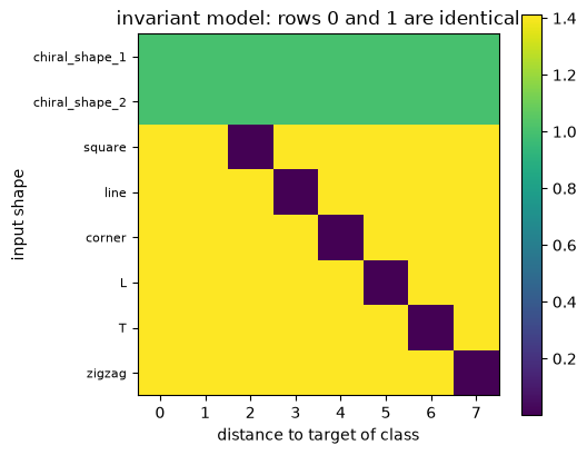
The two top rows of the distance matrix are pixel-identical: whatever class wins for chiral_shape_1 wins for chiral_shape_2 too. Therefore, at least one of them is always wrong (here the model parks both at the loss-minimizing compromise, pseudoscalar-slot \(\approx 0\)). Training longer, wider, or deeper changes nothing: this is a symmetry issue, not an optimization failure.

11.7. Experiment 2: One pseudoscalar in output irreps resolves chirality

We now set the irreps_out to "1x0o + 6x0e". The only change is the parity label of the first entry in the output irreps, which unlocks the 1e \(\otimes\) 1o \(\to\) 0o path in layer 3.

# Set the random seed for reproducibility
torch.manual_seed(1)

# Create an instance of the TetrisNet model with output irreps "1x0o + 6x0e"
# (one pseudoscalar and six true scalars)
model_chi = TetrisNet("1x0o + 6x0e", r_cut, avg_neighbors)
print(f"parameters: {sum(p.numel() for p in model_chi.parameters())}")

# Train the model
hist_chi = train(model_chi)

# Compute the outputs of the model after training
out_chi = model_chi(pos, edge_index, batch, 8)

# Classify the outputs
pred_chi = classify(out_chi)

# Print the results
print(f"final loss {hist_chi[-1]:.2e},  accuracy {accuracy(out_chi):.3f}")
print(f"predictions: {pred_chi.tolist()}")
print(f"pseudoscalar output: chiral_1 -> {out_chi[0,0]:+.3f},  chiral_2 -> {out_chi[1,0]:+.3f}")

# Visualize the training curves for both models
ax = plot_training_curves({"invariant (7x0e)": hist_inv, "chiral (0o + 6x0e)": hist_chi})
ax.set_title("MSE loss: the invariant model hits its symmetry floor")
ax.figure.tight_layout(); plt.show()

parameters: 27941
final loss 4.86e-10,  accuracy 1.000
predictions: [0, 1, 2, 3, 4, 5, 6, 7]
pseudoscalar output: chiral_1 -> -1.000,  chiral_2 -> +1.000

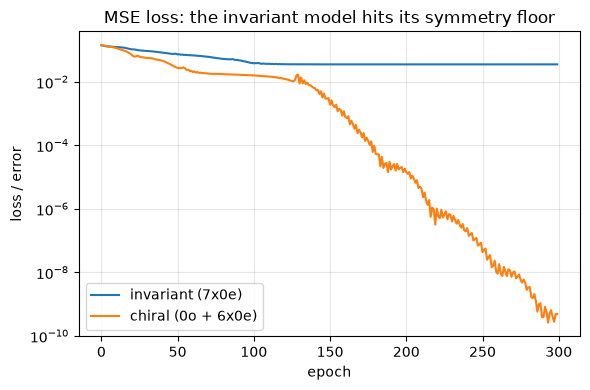
This model achieves 100% classification accuracy and the pseudoscalar comes out equal and opposite on the mirror pair as its transformation law demands. The invariant model’s loss plateaus at exactly the variance it can never explain (\(\tfrac{2 \cdot 1}{8 \cdot 7} \approx 0.036\): the \(\pm 1\) targets of the pair, unreachable, averaged over \(8\times7\) outputs).

11.8. The augmentation-free rotation test

Here, we trained the model on a dataset of shapes in a single orientation. We now, test the network with shapes from the same dataset that have been rotated and translated randomly. Our network should generalize to the rotated dataset as well as it performed on the training and the unrotated test dataset.

# Set the random seed for reproducibility
torch.manual_seed(2)

# Evaluate the model on random rotations and translations of the input shapes
accs = []
for _ in range(20):
    # Generate a random rotation matrix and translation vector
    R, t = o3.rand_matrix(), torch.randn(3)
    
    # Apply the random rotation and translation to the positions of the Tetris shapes
    p_rot, ei_rot, b_rot = batch_graphs([p @ R.T + t for p in pos8], r_cut)
    
    # Compute the accuracy of the model on the rotated and translated shapes
    accs.append(accuracy(model_chi(p_rot, ei_rot, b_rot, 8)))

# Print the mean accuracy over the 20 random rotations and translations ...
print(f"accuracy over 20 random rotations + translations: {np.mean(accs):.3f}")

# ... and the party trick: Invert the shapes -> the chiral pair must swap labels
p_inv, ei_inv, b_inv = batch_graphs([-p for p in pos8], r_cut)
print(f"predictions on inverted shapes: {classify(model_chi(p_inv, ei_inv, b_inv, 8)).tolist()}")
print("  -> shapes 0 and 1 swap (a mirrored left-handed shape IS the right-handed one);")
print("     the 6 achiral shapes are their own mirror images and keep their labels.")

accuracy over 20 random rotations + translations: 1.000
predictions on inverted shapes: [1, 0, 2, 3, 4, 5, 6, 7]
  -> shapes 0 and 1 swap (a mirrored left-handed shape IS the right-handed one);
     the 6 achiral shapes are their own mirror images and keep their labels.

Perfect accuracy under transformations the model has never seen during its training. Furthermore, the model doesn’t fail under inversion applied to the chiral pair: it correctly recognizes that the mirror of shape 0 is shape 1.

Our final sanity check is the full pipeline (positions \(\to\) batched graph \(\to\) 3 convolutions \(\to\) pooled prediction) E(3)-equivariance test performed on the TensorNet with output irreps 1x0o + 6x0e:

assert_model_equivariant(
    lambda p: model_chi(p, edge_index, batch, 8),
    pos, "1x0o + 6x0e",
)

equivariant!  (max error 4.663e-15 over random O(3) + translations elements)

4.6629367034256575e-15

11.9. Summary

• Eight Tetris shapes in the 3D Tetris dataset are batched into one graph and classified end-to-end by a network ofthree TFNConv blocks from Lesson 06a, Gate nonlinearities and a mean-pool readout.

• Parity is expressiveness: an O(3)-equivariant model with only 0e outputs satisfies \(f(-X) = f(X)\) identically for shape \(X\) and its reflection \(-X\). The chiral pair, however, become indistinguishable to the model before and after training (loss floor \(\approx 0.036\), accuracy 75%).

• Declaring one output irrep as a pseudoscalar 0o unlocks the parity chain in 1o \(\otimes\) 1o \(\to\) 1e, and 1e \(\otimes\) 1o \(\to\) 0o paths within three convolutional layers yielding chirality as a triple-product-order feature and a perfect model testing accuracy of 100%.

• Equivariance replaces data augmentation: A TFN trained in one orientation, demonstrates perfect accuracy on random rotations/translations. Under inversion, applied to the chiral pair, the model correctly swaps their classifications, exactly as the label covariance demands.

Next: In Part III, we will build the invariant baseline models: Lesson 07a focuses on SchNet, and Lesson 07b on DimeNet.

11.10. Exercises

1. Ablate the pseudovectors (Difficulty: 🌶️🌶️): In TetrisNet.gate2, remove the 8x1e from the gated irreps (and shrink the gates to 16x0e). Retrain the 1x0o + 6x0e irreps in the output layer of the model. What accuracy do you get, and why exactly?

Solution

Accuracy drops to the invariant model’s 75% and the pseudoscalar output is identically zero: without 1e (or 2o) features in layer 2, layer 3 has no path of total parity o and \(l=0\): FullyConnectedTensorProduct simply finds no instructions ending in 0o. The printed module shows the missing path and the loss plateaus at the same 0.036 floor.

2. Do we need \(l_\mathrm{max} = 2\)? (Difficulty: 🌶️🌶️): Rebuild everything with l_max=1 (spherical harmonics irreps will only have 0e + 1o). Does the chiral model still reach very high testing accuracy? Which paths produce the 1e and 0o now?

Solution

Yes. It will achieve the same accuracy, but more slowly. Here, the 1e irrep only comes from the 1o \(\otimes\) 1o \(\to\) 1e (the cross product) in layer 2, and the 0o irrep comes from the 1e \(\otimes\) 1o \(\to\) 0o (the triple product) in layer 3: exactly the two paths the original TFN code implements from scratch (\(\epsilon_{ijk}\) and the dot product). With l_max=2 there are extra parity-odd routes: layer 2 can also build 2o (via 1o \(\otimes\) 2e \(\to\) 2o), which layer 3 closes with 2o \(\otimes\) 2e \(\to\) 0o. So, we get more paths into the pseudoscalar, favoring a faster training. We recommend trying steps=600 for a reliable classification training at l_max=1.

3. Prove the loss floor (Difficulty: 🌶️🌶️🌶️): Show that for any inversion-invariant predictor \(f\), the minimum of the MSE loss over the 8 shapes is \(2/(8 \cdot 7)\), attained when the pseudoscalar slot predicts \(0\) for the chiral pair.

Solution

The train() function minimizes the MSE loss, which is the mean of \(8 \times 7 = 56\) squared errors: one per shape \(k\) and output slot \(c\):

(2)\[ \mathcal{L} = \frac{1}{56} \sum_{k=0}^{7} \sum_{c=0}^{6} \bigl[ f_c(X_k) - t_{kc} \bigr]^2, \]

where \(t_{kc}\) are the entries of the target table from the Targets section.

Inversion-invariance adds exactly one constraint. Since shape 1 is the inversion of shape 0 (\(X_1 = -X_0\), up to a rotation), an invariant model must return the same 7 numbers for both: \(f_c(X_0) = f_c(X_1)\) for every slot \(c\). The other six shapes are not tied to anything. Now go through the 56 terms and ask which ones this constraint prevents from reaching zero:

• Shapes 2-7 (\(6 \times 7 = 42\) terms): Terms are unconstrained. So, a sufficiently expressive model drives all of these errors to zero (and the trained model in Experiment 1 indeed does. Here, the model can classify these six shapes perfectly).

• Shapes 0/1, slots 1-6 (\(2 \times 6 = 12\) terms): the model is forced to output equal values for the pair. But the targets in these slots are also equal (all zeros). So, the quality costs nothing. These errors also reach zero.

• Shapes 0/1, slot 0 (2 terms): here the targets are \(-1\) and \(+1\), yet the model must answer with a single common value \(y = f_0(X_0) = f_0(X_1)\). The best compromise is found by minimizing this slot’s contribution over \(y\):

  (3)\[ \min_y \bigl[ (y - (-1))^2 + (y - (+1))^2 \bigr] = \min_y \bigl[ 2y^2 + 2 \bigr] = 2, \quad \text{attained at } y = 0. \]

Adding the three groups, the smallest achievable sum of squared errors is \(0 + 0 + 2 = 2\), so the minimum mean is \(\mathcal{L}_\text{min} = 2/56 \approx 0.0357\). This is precisely the plateau of the invariant model’s curve in the training loss figure and, as predicted, its pseudoscalar slot arrives at \(y = 0\) for both chiral shapes.

11.11. References

• e3nn MRS Fall 2021 tutorial

• Geiger & Smidt, e3nn: Euclidean Neural Networks arXiv.2207.09453 (2021)

• Thomas et al., Tensor Field Networks arXiv.1802.08219 (2018)