13. Lesson 07b: DimeNet and the insufficiency of distance-only GNNs

What you will learn

• A concrete, runnable example from two genuinely different structures that no distance-based graph neural network (GNN), including SchNet, at any cutoff, can distinguish.

• Directional message passing: Embeddings that live on directed edges, \(m_{ji}\), instead of atoms, are updated using the angles between edges, while the prediction stays invariant.

• DimeNet’s physically motivated Bessel radial basis and 2D spherical Fourier-Bessel basis, alongside the DimeNet++ efficiency fixes.

• A simplified, educational DimeNet-style model (simplifications stated explicitly), trained on the same LJ-argon data as Lesson 07a. We will discuss the reasons behind the small gain here.

• The cost of feature triplets: \(O(Nk^2)\) vs. \(O(Nk)\). This is our motivation for Part IV’s equivariant approach.

Prerequisites:

• Lesson 07a: SchNet, forces from autograd, the training pipeline (reused here),

• Lesson 05b: Radial bases and cutoffs.

import sys
sys.path.insert(0, "..")    # Make course_utils importable

import copy, time, warnings
import numpy as np
import torch
import torch.nn as nn
import matplotlib.pyplot as plt
from e3nn import o3

from course_utils.data import make_lj_argon_dataset, train_val_split, radius_graph
from course_utils.plotting import (plot_training_curves, scene3d,
                                    draw_point_cloud, show3d)
from course_utils.equivariance import assert_model_equivariant

warnings.filterwarnings("ignore", category=FutureWarning)  # ASE Langevin deprecation notice
torch.manual_seed(0)
np.random.seed(0)
device = "cuda" if torch.cuda.is_available() else "cpu"
silu = nn.functional.silu          # "swish" σ(x) = x·sigmoid(x), DimeNet's activation
print(f"device = {device}, torch {torch.__version__}")

device = cuda, torch 2.7.1+cu126

13.1. Distance-based GNNs are incomplete

Lesson 07a’s SchNet sees a molecule only through its atom types and pairwise distances: a distance-graph NN (dGNN). Message passing makes such models surprisingly powerful. That is, after two message passing iterations, an atom “knows” about not only its own interatomic distances but its neighbors’ distances too, which is often enough to reconstruct the angles implicitly.

Pozdnyakov & Ceriotti analyze dGNNs with a distance-decorated Weisfeiler–Lehman (WL) test. Here, they iteratively re-label each node by the hash

(1)\[ h_i = \mathrm{hash}\big(l_i,\ \{\!\{\,(l_j, r_{ij})\,\}\!\}_{j=1}^{n}\big), \]

where \(l_i\) is the node label, \(r_{ij}\) the distance, and \(\{\!\{\cdot\}\!\}\) a multiset (an unordered set with repetition). If two structures produce identical multisets of hashes at every iteration, no dGNN can ever distinguish them, regardless of weights, depth, or training. This manuscript presents a family of structure pairs, \(\mathcal{A}^\pm\), that are distinct (different angle sets, and different physics) yet WL-indistinguishable for any cutoff, even fully connected.

13.1.1. How the counterexample is built

Start with an infinite chain of identical atoms that repeats with period \(p\) along the \(x\)-axis. Each repeating unit contains six points, arranged in three pairs that we label \((C, C')\), \((V, V')\) and \((W, W')\). The two members of each pair are related by the same operation: shift by half a period along \(x\) and mirror in \(z\),

(2)\[ q = (x, y, z) \;\longmapsto\; q' = \big(x + \tfrac{p}{2},\ y,\ -z\big). \]

The \(V\) pair lies in the \(z = 0\) plane and the \(W\) pair sits at height \(\pm w_z\): both are the same in the two structures. The only difference between \(\mathcal{A}^+\) and \(\mathcal{A}^-\) is the sign of the \(z\)-coordinate of the \(C\) pair; that is \(C = (p/4,\, c_y,\, \pm c_z)\).

Why does this flip preserve every distance? Because \(C\) sits exactly halfway between \(W\) and its shifted-and-mirrored partner \(W'\) along \(x\), sending \(c_z \to -c_z\) simply swaps the two distances: the distance from \(C\) to \(W\) in \(\mathcal{A}^+\) equals the distance from \(C\) to \(W'\) in \(\mathcal{A}^-\), and vice versa (the same happens for \(C'\)). Every atom therefore sees exactly the same multiset of neighbor distances in both structures. As such, the WL hashes agree at every iteration. The angles, however, change, so that the two structures become genuinely different shapes with different physics.

An infinite chain is not a molecule, so the last step makes the pair finite: we take \(P\) consecutive periods of the chain (here \(P = 2\)) and wrap them into a closed ring around the \(z\)-axis, turning \(x\) into a polar angle \(\theta = 2\pi x /(pP)\) and \(y\) into a small radial offset from a ring of radius \(pP/2\pi\). The result is two finite clouds of \(6P = 12\) points each that inherit the distance degeneracy (we verify this numerically below). Pozdnyakov & Ceriotti show that such pairs can even be realized as configurations of four water molecules. Let’s build the folded pair and check everything numerically.

def degenerate_pair(p=6.0, c_y=0.2, c_z=0.8, v_x=1.1, v_y=-0.4, w_y=0.6, w_z=1.3, P=2):
    '''Pozdnyakov & Ceriotti (2022): A+/A- pair'''
    
    # Primed = (p/2 + x, y, -z)
    def unit_cell(sign):
        C = (p / 4, c_y, sign * c_z)
        W = (p / 2, w_y, w_z)
        V = (v_x, v_y, 0.0)
        prime = lambda q: (p / 2 + q[0], q[1], -q[2])
        return [C, prime(C), V, prime(V), W, prime(W)]
    
    # Wrap P periods around z
    def fold(points):
        out = []
        for k in range(P):
            for (x, y, z) in points:
                theta = 2 * np.pi * (x + k * p) / (p * P)
                r = P * p / (2 * np.pi) + y
                out.append((r * np.cos(theta), r * np.sin(theta), z))
        return torch.tensor(out, dtype=torch.float64)
    
    # Return the two structures A+ and A- as torch tensors of shape (6*P, 3) 
    return fold(unit_cell(+1)), fold(unit_cell(-1))

# Generate the two structures and print their sizes
A_plus, A_minus = degenerate_pair()
print("two finite structures with", len(A_plus), "points each")

two finite structures with 12 points each

# Sorted list of all pair distances
def distance_multiset(pos):
    d = torch.cdist(pos, pos)
    iu = torch.triu_indices(len(pos), len(pos), offset=1)
    return d[iu[0], iu[1]].sort().values

# Sorted cos(angle) over all triplets i-j-k
def angle_multiset(pos):
    # vecs[j, i] = r_i - r_j
    vecs = pos.unsqueeze(0) - pos.unsqueeze(1)
    n = len(pos); cos = []
    for j in range(n):
        for i in range(n):
            for k in range(i + 1, n):
                if i == j or k == j: continue
                u, v = vecs[j, i], vecs[j, k]
                cos.append((u @ v / (u.norm() * v.norm())).item())
    return torch.tensor(sorted(cos))

# Compare the two structures
dd = (distance_multiset(A_plus) - distance_multiset(A_minus)).abs().max()
da = (angle_multiset(A_plus) - angle_multiset(A_minus)).abs().max()
print(f"pair-distance multisets:  max difference = {dd:.2e}   (identical)")
print(f"angle multisets:          max difference = {da:.2e}   (DIFFERENT -> distinct shapes)")

pair-distance multisets:  max difference = 8.88e-16   (identical)
angle multisets:          max difference = 1.64e-01   (DIFFERENT -> distinct shapes)

# Visualize the two structures
labels = ["C", "C'", "V", "V'", "W", "W'"]
colors = ["C0", "C0", "C1", "C1", "C2", "C2"]
symbols = ["circle", "diamond", "circle", "diamond", "circle", "diamond"]

# The two environments differ only in angles, so rotate them to see it
fig = scene3d(1, 2, titles=["A+  (same distances, different angles)",
                            "A-  (same distances, different angles)"], title_dy=-0.05)
for panel, pos in enumerate([A_plus, A_minus]):
    for t in range(6):                                    # 6 point types, P=2 copies each
        draw_point_cloud(pos[t::6], fig=fig, cell=(1, panel + 1), color=colors[t],
                         symbol=symbols[t], size=7,
                         label=labels[t] if panel == 0 else None)
show3d(fig, axes=True)

13.1.2. A dGNN really cannot tell them apart

The WL test is architecture-independent. As such, we can demonstrate it with a random, untrained distance-based message-passing network: If the two structures produced different outputs for any weights, they would be WL-distinguishable.

We use a fully connected graph (cutoff larger than the biggest distance), the hardest case for the counterexample, and it still holds.

class MiniDGNN(nn.Module):
    '''A generic distance-based MPNN (the SchNet blueprint), random weights, float64.'''
    
    # We use a fully connected graph (cutoff larger than the biggest distance)
    def __init__(self, F=32, n_rbf=16, r_max=10.0):
        super().__init__()
        # Create a grid of radial basis function centers, evenly spaced in [0, r_max]
        self.register_buffer("mu", torch.linspace(0.0, r_max, n_rbf))
        
        # Message function: takes in a node feature vector and a radial basis
        # function vector, outputs a new node feature vector
        self.msg = nn.Sequential(nn.Linear(F + n_rbf, F), nn.Tanh(), nn.Linear(F, F))
        
        # Readout function: takes in a node feature vector and outputs a scalar energy
        self.readout = nn.Linear(F, 1)
        
        # Number of features per node
        self.F = F
    
    # Forward pass: compute the "energy" of a point cloud
    def forward(self, pos):
        # Fully connected graph here
        i, j = radius_graph(pos, r_cut=10.0)
        
        # Compute the radial basis functions
        e = torch.exp(-10.0 * ((pos[j] - pos[i]).norm(dim=-1, keepdim=True) - self.mu) ** 2)
        
        # One species -> identical init
        x = torch.ones(len(pos), self.F, dtype=pos.dtype)
        
        # 3 rounds of message passing
        for _ in range(3):
            m = self.msg(torch.cat([x[j], e], dim=-1))
            x = x + torch.zeros_like(x).index_add_(0, i, m)
        
        # Readout: sum over all nodes
        return self.readout(x).sum()

# Initialize the dGNN and compute energies for both structures
dgnn = MiniDGNN().double()
E_p, E_m = dgnn(A_plus).item(), dgnn(A_minus).item()
print(f"dGNN(A+) = {E_p:.12f}\ndGNN(A-) = {E_m:.12f}\ndifference = {abs(E_p - E_m):.2e}")

dGNN(A+) = -28.836528410246
dGNN(A-) = -28.836528410246
difference = 7.11e-15

Identical energies to machine precision! This observation holds for every weight setting, every depth, every cutoff. The fix suggested by the paper’s is to use the angular information: 3-body descriptors, or GNNs such as DimeNet/GemNet that pass messages between edges. That is directional message passing.

13.2. Directional message passing (DimeNet)

Classical force fields decompose the energy as:

(3)\[ E = E_\text{bonds} + E_\text{angle} + E_\text{torsion} + E_\text{non-bonding}, \]

where \(E_\text{bonds}\), \(E_\text{angle}\), \(E_\text{torsion}\), and \(E_\text{non-bonding}\) are the energy contributions from bonds, angles, torsions (i.e., rotations around bonds based on dihedral angles), and non-bonded interactions (i.e., van der Waals and electrostatic interactions), respectively. Noting that a standard message-passing GNN updates the atom \(i\)’s features in layer \(l\), \(h_i^{(l)}\), using an update function,\(f_\text{update}\), of the form,

(4)\[ h_i^{(l+1)} = f_\text{update}\Big(h_i^{(l)}, \sum_{j \in \mathcal{N}_i} f_\text{int}\big(h_j^{(l)}, e^{(l)}_{(ij)}\big)\Big) \]

it only sees the distance-based edge embeddings, \(e^{(l)}_{(ij)}\). As such, the predicted total energy of the model lacks the angle, torsion and the non-bonding terms. Both update and interaction functions, \(f_\text{update}\) and \(f_\text{int}\), are often implemented as neural networks.

The DimeNet’s main idea is to embed the directed edges alongside the atomic embeddings. The message embedding, \(m_{ji} \in \mathbb{R}^F\), is associated with the atom pair \(j \to i\). The atomic embedding is recovered as the sum of its incoming messages, \(h_i = \sum_{j \in \mathcal{N}_i} m_{ji}\). Each message is tied to a direction in space, and directions rotate with the molecule. Thus, relative directional information (angles) between messages is preserved, while the network only ever consumes invariant scalars: distances and angles.

A message \(m_{ji}\) is updated from the messages \(m_{kj}\) flowing into its source atom \(j\) (excluding the one coming back from \(i\)), using the angle \(\alpha^{(kj,ji)} = \angle\, \vec x_k\, \vec x_j\, \vec x_i\) between the two edges at the vertex \(j\). Thus, the directional message-passing equation can be written as

(5)\[ m_{ji}^{(l+1)} = f_\text{update}\Big( m_{ji}^{(l)}, \sum_{k \in \mathcal{N}_j \setminus \{i\}} f_\text{int}\big( m_{kj}^{(l)},\, e_\mathrm{RBF}^{(ji)},\, a_\mathrm{SBF}^{(kj,ji)} \big) \Big), \]

where \(e_\mathrm{RBF}^{(ji)}\) is a radial-basis representation of \(d_{ji}\) and \(a_\mathrm{SBF}^{(kj,ji)}\) is a joint 2D basis of \(\big(d_{kj},\, \alpha^{(kj,ji)}\big)\). This aggregation over pairs of edges, triplets \((k, j, i)\) of atoms, is what lets the model learn the \(E_\text{angle}\) directly. Consequently, the model can distinguish among structures (like the \(\mathcal{A}^+/\mathcal{A}^-\) pair above) that lead to the failure of every dGNN. Message embeddings are pair embeddings, connecting DimeNet to the provably more expressive higher-order WL hierarchies.

13.2.1. Bessel radial basis and the 2D spherical Fourier–Bessel basis

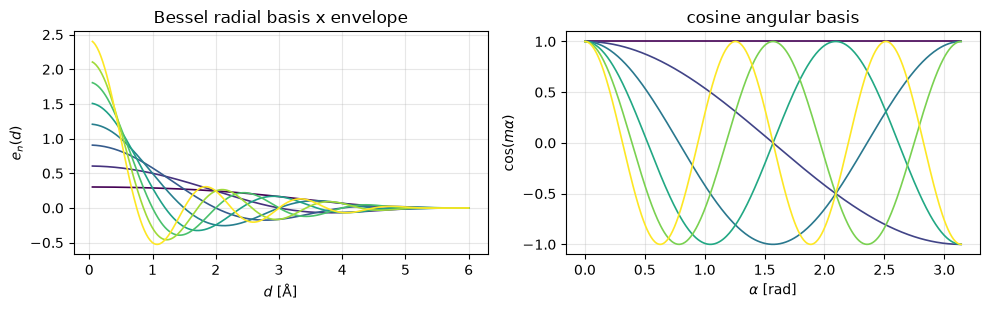
Instead of Gaussians (Lesson 07a), DimeNet derives its bases from the free Schrödinger/Helmholtz equation inside a sphere with a cutoff radius, \(c\), and the boundary condition, \(\Psi(c) = 0\). The 1D radial Bessel basis for \(d_{ji}\), expressed as

(6)\[ \tilde e_\mathrm{RBF,n}(d) = \sqrt{\frac{2}{c}}\, \frac{\sin\!\big(\tfrac{n_1\pi}{c} d\big)}{d}, \qquad n_1 \in \{1, 2, \ldots, N_\mathrm{RBF}\}, \]

are real-valued andorthogonal with a bounded maximum frequency \(n_1\pi/c\) (a built-in regularizer). The radial Bessel functions match the accuracy of Gaussian-RBFs with \(4\)–\(20\times\) fewer basis functions. The joint 2D spherical Fourier-Bessel basis, \(\tilde a_\mathrm{SBF,ln}(d, \alpha) \in \mathbb{R}^{N_\mathrm{SHBF} \times N_\mathrm{SRBF}}\), combines spherical Bessel functions, \(j_l\), with spherical harmonics, \(Y_l^0\):

(7)\[ \tilde a_\mathrm{SBF,ln_2}(d, \alpha) = \sqrt{\frac{2}{c^3\, j_{l+1}^2(z_{ln_2})}}\; j_l\!\Big(\frac{z_{ln_2}}{c} d\Big)\, Y_l^0(\alpha), \qquad n_2 \in \{1, 2, \ldots, N_\mathrm{SRBF}\}, \qquad \text{and} \qquad l \in \{0, 1, \ldots, N_\mathrm{SHBF}-1\} \]

where \(z_{ln}\) (dropping the subscript) is the \(n\)-th root of \(l\)-th-order Bessel function, \(j_l\). Both bases are multiplied by a smooth envelope \(u(d)\) with a root of multiplicity 3 at the cutoff. With \(p = 6\), \(d\) in units of \(c\), one can write

(8)\[ u(d) = 1 - \frac{(p+1)(p+2)}{2} d^{p} + p(p+2)\, d^{p+1} - \frac{p(p+1)}{2} d^{p+2}. \]

Thus, the model becomes twice continuously differentiable, \(\mathcal{C}^2\), which is a desired property for training machine learning models on forces. The embedding block initializes messages from the endpoint atom embeddings and the distance as:

(9)\[ m_{ji}^{(1)} = \mathrm{SiLU}\big( [\, h_j^{(0)}\, \Vert\, h_i^{(0)}\, \Vert\, e_\mathrm{RBF}^{(ji)}\,] W + b \big), \]

where \(\Vert\) denotes concatenation and \(\mathrm{SiLU}\) is a self-gated Swish or sigmoid linear unit (SiLU) activation function, defined as

(10)\[ \mathrm{SiLU}(x) = x \cdot \sigma(x). \]

13.2.2. DimeNet++

The DimeNet++ model keeps a similar architecture design as DimeNet but replaces the expensive bilinear triplet layer with a Hadamard (element-wise) product plus small multi-layer perceptrons (MLP) on the basis representations, adds down-/up-projections of the embeddings, and uses 4 instead of 6 interaction blocks leading to 8× faster and ~10 % more accurate performance on the QM9 benchmark set.

13.2.3. A pedagogical instance of DimeNet++

Here, we implement the ideas faithfully but keep the code simple and small. We explicitly state the simplifications vs. the original DimeNet and DimeNet++ papers:

1. 2D basis \(\to\) separable product. Instead of the spherical Fourier-Bessel basis, we use the product

   (11)\[ a^{(kj,ji)}_{nm} = e_{\mathrm{RBF},n}(d_{kj}) \cdot \cos\!\big(m\,\alpha^{(kj,ji)}\big) \]

   That is, the radial Bessel basis of in \(d_{kj}\) times a cosine basis in the angle. Our choice is informed by the fact that \(Y_l^0(\alpha) \propto P_l(\cos\alpha)\). Thus, a smooth polynomial basis in \(\cos\alpha\) plays the same role and both choices can span the same function space as their order grows.

2. Hadamard interaction instead of a bilinear one: This is the DimeNet++’s simplification.

3. Slimmer architecture: We adopt 2 interaction blocks, \(F = 64\), one readout at the end. In comparison, the original DimeNet model uses 6 blocks with residual sub-blocks and a per-block output that is summed (\(t = \sum_i \sum_l t_i^{(l)}\)). The DimeNet++ model uses 4 blocks with down-/up-projections.

4. Fixed Bessel frequencies \(k_n = n\pi/c\). The DimeNet paper fine-tunes them during training using backpropagation. We keep them fixed to avoid the extra complexity and reduce the computational cost.

5. Same training setup as Lesson 07a: We use the same loss, optimizer, standardization, full batch setup. So, the two models (SchNet and DimeNet) are compared as apples-to-apples. DimeNet’s own MD loss is the same energy + \(\rho\)-weighted force combination we quoted from the SchNet manuscript in Lesson 07a.

We compute \(\cos(m\alpha)\) from \(\cos\alpha\) via the Chebyshev recursion \(T_m(\cos\alpha) = \cos(m\alpha)\), \(T_m(x) = 2x\,T_{m-1}(x) - T_{m-2}(x)\). This choice avoids computing the \(\arccos\) function, whose derivative blows up at collinear triplets (\(\alpha \in \{0, \pi\}\)) and would poison the force gradients.

Let us implement our pedagogical DimeNet++ and train it on the same LJ-argon data as Lesson 07a. The first part is the implementation of the Bessel radial basis as well as the cosine basis functions via Chebyshev recursion.

# Create the Bessel radial basis functions (RBFs) with a smooth cutoff
class BesselRBF(nn.Module):
    '''e_n(d) = u(d/c) * sqrt(2/c) sin(n pi d / c) / d'''
    
    def __init__(self, r_cut: float, n_rbf: int = 8, p: int = 6):
        super().__init__()
        self.register_buffer("n", torch.arange(1, n_rbf + 1, dtype=torch.get_default_dtype()))
        self.r_cut, self.p = r_cut, p

    # x = d / c in [0, 1]
    def envelope(self, x):
        p = self.p
        return (1 - (p + 1) * (p + 2) / 2 * x**p + p * (p + 2) * x**(p + 1)
                - p * (p + 1) / 2 * x**(p + 2))

    # (E,) -> (E, n_rbf)
    def forward(self, d):
        x = (d / self.r_cut).unsqueeze(-1)
        e = np.sqrt(2.0 / self.r_cut) * torch.sin(self.n * np.pi * x) / d.unsqueeze(-1)
        return e * self.envelope(x)

# Create the cosine basis functions via Chebyshev recursion
def cos_basis(cos_alpha, n_ang: int):
    '''[T_0, ..., T_{n_ang-1}](cos a) = [1, cos a, cos 2a, ...] via Chebyshev recursion.'''
    T = [torch.ones_like(cos_alpha), cos_alpha]
    for _ in range(n_ang - 2):
        T.append(2 * cos_alpha * T[-1] - T[-2])
    # (T, n_ang)
    return torch.stack(T[:n_ang], dim=-1)

We can now visualize the Bessel radial basis functions and the cosine basis functions

# Create the figure and axes for the plots
fig, (ax1, ax2) = plt.subplots(1, 2, figsize=(10, 3.2))

# Create a grid of distances and compute the Bessel radial basis functions
d = torch.linspace(0.05, 6.0, 400)
eb = BesselRBF(6.0)(d)

# Plot the Bessel radial basis functions
colors = plt.get_cmap("viridis")(np.linspace(0, 1, eb.shape[1]))   # sequential: ordered n
for k in range(eb.shape[1]):
    ax1.plot(d, eb[:, k], color=colors[k], lw=1.2)
ax1.set_xlabel(r"$d$ [Å]"); ax1.set_ylabel(r"$e_n(d)$")
ax1.set_title("Bessel radial basis x envelope"); ax1.grid(True, alpha=0.3)

# Create a grid of angles and compute the cosine basis functions
alpha = torch.linspace(0, np.pi, 400)
cb = cos_basis(torch.cos(alpha), 6)

# Plot the cosine basis functions
colors = plt.get_cmap("viridis")(np.linspace(0, 1, cb.shape[1]))
for m in range(cb.shape[1]):
    ax2.plot(alpha, cb[:, m], color=colors[m], lw=1.2)
ax2.set_xlabel(r"$\alpha$ [rad]"); ax2.set_ylabel(r"$\cos(m\alpha)$")
ax2.set_title("cosine angular basis"); ax2.grid(True, alpha=0.3)
fig.tight_layout()

13.2.4. Triplets

The directed edges are given by edge_index (receiver \(i\), sender \(j\): Lesson 05a convention). A triplet represents a pair of edges, \((k \to j,\ j \to i)\), with \(k \neq i\). As a result, the message, \(m_{kj}\), feeds the update of \(m_{ji}\). We find all such pairs once per (static) training set with a dense comparison: It’s memory cost is \(O(E^2)\) which is fine for our course’s tiny graphs. However, the production codes use more efficient sorted/CSR neighbor lists. The angle at vertex \(j\) is computed in the forward pass from positions (it must stay in the autograd graph). The cosine of the angle is computed as

(12)\[ \cos\alpha^{(kj,ji)} = \frac{(\vec x_k - \vec x_j) \cdot (\vec x_i - \vec x_j)} {\lVert \vec x_k - \vec x_j \rVert\, \lVert \vec x_i - \vec x_j \rVert}. \]

def find_triplets(edge_index):
    '''All edge pairs (a: k->j, b: j->i) with k != i. Returns (a_idx, b_idx) into edges.'''
    
    # Edge e: send[e] -> recv[e]
    recv, send = edge_index
    
    # a's receiver j == b's sender j
    match = recv.unsqueeze(1) == send.unsqueeze(0)
    
    # a's sender k != b's receiver i
    not_backtrack = send.unsqueeze(1) != recv.unsqueeze(0)
    
    # Return the indices of the triplet edges
    a_idx, b_idx = (match & not_backtrack).nonzero(as_tuple=True)
    return a_idx, b_idx

# Sanity check on one frame
_pos = make_lj_argon_dataset(n_frames=1)[0]["pos"]
_ei = radius_graph(_pos, 6.0)
_a, _b = find_triplets(_ei)
print(f"frame with {_ei.shape[1]} directed edges -> {len(_a)} triplets")

frame with 30 directed edges -> 96 triplets

13.2.5. The model

Each interaction block in our DimeNet+±style model involves a Hadamard multiplication in the interaction function, \(f_\text{int}\), followed by a residual update function, \(f_\text{update}\):

(13)\[ s_{ji} = \sum_{k \in \mathcal{N}_j \setminus \{i\}} f_\text{int}(\cdot), \]

(14)\[ f_\text{int}\big(m_{kj}, e^{(ji)}, a^{(kj,ji)}\big) = \big(W_e\, e_\mathrm{RBF}^{(ji)}\big) \odot \big(W_a\, a_\mathrm{SBF}^{(kj,ji)}\big) \odot \mathrm{SiLU}\big(W_m\, m_{kj}\big), \]

(15)\[ m^{(l+1)}_{ji} = f_\text{update}(m^{(l)}_{ji}, s_{ji}) = m^{(l)}_{ji} + \mathrm{SiLU}\big(W_2\, \mathrm{SiLU}(W_1 [\, m^{(l)}_{ji} \Vert s_{ji}\,])\big). \]

Then, the readout yields the updated the atomic features via messages \(h_i = \sum_j m_{ji},\) and atom-wise dense layers use them to yield a per-atom energy, summed to \(\hat E\).

Let us implement this in code:

class DirectionalInteraction(nn.Module):
    """A directional interaction block in the DimeNet++ architecture."""
    
    def __init__(self, F: int, n_rbf: int, n_ang: int):
        super().__init__()
        # Gate by e_RBF(d_ji)
        self.W_e = nn.Linear(n_rbf, F, bias=False)
            
        # Filter from joint (d_kj, angle) basis
        self.W_a = nn.Linear(n_rbf * n_ang, F, bias=False)
        
        # Transform incoming message m_kj
        self.W_m = nn.Linear(F, F)
        
        # Residual update
        self.W_1 = nn.Linear(2 * F, F)
        self.W_2 = nn.Linear(F, F)

    # f_int: Hadamard product over each triplet (k->j, j->i)
    def forward(self, m, e, a, trip_a, trip_b):
        # Compute the message for each triplet (k->j, j->i)    
        t = self.W_e(e)[trip_b] * self.W_a(a) * silu(self.W_m(m[trip_a]))
        
        # Sum over k in N(j)\{i}
        s = torch.zeros_like(m).index_add_(0, trip_b, t)
        
        # f_update
        return m + silu(self.W_2(silu(self.W_1(torch.cat([m, s], dim=-1)))))

class SimpleDimeNet(nn.Module):
    """A simple DimeNet++ model for energy prediction."""
    
    def __init__(self, n_features=64, n_blocks=2, r_cut=6.0, n_rbf=8, n_ang=6, n_species=1):
        super().__init__()
        # Create the Bessel radial basis functions
        self.rbf = BesselRBF(r_cut, n_rbf)
        
        # Embedding for atomic species
        self.embedding = nn.Embedding(n_species, n_features)
        
        # Edge embedding: concatenates h_i, h_j, and e_RBF(d_ji) to produce m_ji
        self.edge_embed = nn.Linear(2 * n_features + n_rbf, n_features)
        
        # Create a stack of directional interaction blocks
        self.blocks = nn.ModuleList(
            [DirectionalInteraction(n_features, n_rbf, n_ang) for _ in range(n_blocks)])
        
        # Readout: two dense layers to produce a per-atom energy
        self.readout1 = nn.Linear(n_features, n_features // 2)
        self.readout2 = nn.Linear(n_features // 2, 1)
        
        # Number of angular basis functions
        self.n_ang = n_ang

    # Forward pass: compute the energy of a point cloud
    def forward(self, pos, species, edge_index, trip_a, trip_b, batch, n_graphs):
        # Edge index: recv = j, send = i for each edge j->i
        recv, send = edge_index
        
        # Compute d_ji: distance from atom j to atom i
        d = (pos[send] - pos[recv]).norm(dim=-1)
        
        # Compute the radial basis functions
        e = self.rbf(d)
        
        # Compute the initial node features h_i from the atomic species
        h = self.embedding(species)
        
        # Compute the edge features m_ji
        m = silu(self.edge_embed(torch.cat([h[send], h[recv], e], dim=-1)))
        
        # x_k - x_j
        u = pos[send[trip_a]] - pos[recv[trip_a]]
        
        # x_i - x_j
        v = pos[recv[trip_b]] - pos[send[trip_b]]
        
        # Compute the cosine of the angle alpha between u and v
        cos_alpha = (u * v).sum(-1) / (u.norm(dim=-1) * v.norm(dim=-1))
        
        # e_RBF(d_kj) x cos(m alpha)
        a = (self.rbf(u.norm(dim=-1)).unsqueeze(-1)
             * cos_basis(cos_alpha, self.n_ang).unsqueeze(-2)).flatten(-2)
        
        # Apply the directional interaction blocks
        for block in self.blocks:
            m = block(m, e, a, trip_a, trip_b)
        
        # h_i = sum_j m_ji
        h_i = torch.zeros(len(pos), m.shape[-1], dtype=pos.dtype,
                          device=pos.device).index_add_(0, recv, m)
        
        # Readout: compute the per-atom energies E_i and sum over all atoms in each graph
        E_i = self.readout2(silu(self.readout1(h_i))).squeeze(-1)
        E = torch.zeros(n_graphs, dtype=pos.dtype, device=pos.device)
        
        # E = sum_i E_i
        return E.index_add_(0, batch, E_i)

Let’s initilize the model and print the number of parameters.

model = SimpleDimeNet().to(device)
print("SimpleDimeNet parameters:", sum(p.numel() for p in model.parameters()))

SimpleDimeNet parameters: 51265

13.2.6. Does it resolve the counterexample?

Before we proceed with training our DimeNet++ model, let’s perform another experiment with \(\mathcal{A}^+/\mathcal{A}^-\) pair, again with random untrained weights: if the architecture carries angular information, as it does in the case of DimeNet++, the two structures should already map to different outputs.

# Fully connected graph at r_cut = 10 Å
dime64 = SimpleDimeNet(r_cut=10.0).double()

# Compute the energies of the two structures using the float64 DimeNet model
def dime_energy(pos):
    ei = radius_graph(pos, 10.0)
    ta, tb = find_triplets(ei)
    z = torch.zeros(len(pos), dtype=torch.long); b = torch.zeros(len(pos), dtype=torch.long)
    return dime64(pos, z, ei, ta, tb, b, 1).item()

E_p, E_m = dime_energy(A_plus), dime_energy(A_minus)
print(f"SimpleDimeNet(A+) = {E_p:.8f}\nSimpleDimeNet(A-) = {E_m:.8f}")
print(f"difference = {abs(E_p - E_m):.3e}   <- angles break the degeneracy")

SimpleDimeNet(A+) = 9.54261730
SimpleDimeNet(A-) = 9.54456491
difference = 1.948e-03   <- angles break the degeneracy

13.3. Training on LJ argon and a comparison with SchNet

This section is set up with the same data, split, standardization, loss (\(\rho = 1\)), optimizer and schedule as Lesson 07a. Forces from autograd are obtained exactly as before. The only new ingredient in the pipeline is the precomputed triplet list per batch.

It is important to note that the Lennard-Jones (LJ) expression is a pure pair potential where the energy is a function of distances only:

(16)\[ E = \sum_{i<j} 4\varepsilon\big[(\sigma/d_{ij})^{12} - (\sigma/d_{ij})^{6}\big]. \]

Here, \(\varepsilon\) is the depth of the potential well and \(\sigma\) is the distance at which the potential is zero. The LJ potential is perfectly representable by a distance-based model. Adding the angular features add no missing physics on the L-J argon dataset. As such, we expect no gains from a DimeNet-style mode. We proceed with training our model on this data regardless, in order to validate the implementation and set the stage for Lesson 07c, where we will train on a dataset with genuine angular information.

Angular information matters also when the target actually depends on it: covalent/directional bonding (the water bend, \(sp^3\) angles, torsions etc.), many-body metals and semiconductors (e.g. silicon phases), and whenever distance-degenerate configurations occur (e.g., in the case of cyclic molecules).

# Create the LJ-argon dataset
frames = make_lj_argon_dataset(n_frames=200, n_atoms=8, seed=0)

# Split into training and validation sets
train_frames, val_frames = train_val_split(frames, val_fraction=0.25, seed=0)

# Get the number of atoms
n_atoms = frames[0]["pos"].shape[0]

# Compute the per-atom mean shift (see Lesson 07a)
E_train = np.array([f["energy"] for f in train_frames])
eps_bar = E_train.mean() / n_atoms

# Set the cutoff radius for the graph construction
R_CUT = 6.0

# Make a batch of graphs from a list of frames
def make_batch(frame_list, device):
    '''One disconnected graph: pos, species, edges, triplets, batch, E~, F.'''
    
    pos, species, edges, batch, E, F = [], [], [], [], [], []
    offset = 0
    for g, f in enumerate(frame_list):
        p = f["pos"].float()
        pos.append(p)
        species.append(torch.zeros(len(p), dtype=torch.long))
        edges.append(radius_graph(p, R_CUT) + offset)
        batch.append(torch.full((len(p),), g, dtype=torch.long))
        E.append(f["energy"] - len(p) * eps_bar); F.append(f["forces"].float())
        offset += len(p)
    edge_index = torch.cat(edges, dim=1)
    
    # Precompute the triplets for the entire batch (static geometry)
    trip_a, trip_b = find_triplets(edge_index)
    return (torch.cat(pos).to(device), torch.cat(species).to(device),
            edge_index.to(device), trip_a.to(device), trip_b.to(device),
            torch.cat(batch).to(device),
            torch.tensor(E, dtype=torch.float32, device=device), torch.cat(F).to(device))

# Make a batch of graphs for training and validation
train_batch = make_batch(train_frames, device)
val_batch   = make_batch(val_frames, device)

# Print the number of frames and the graph statistics
print(f"{len(train_frames)} train / {len(val_frames)} val frames | train graph: "
      f"{train_batch[0].shape[0]} atoms, {train_batch[2].shape[1]} edges, {len(train_batch[3])} triplets")

150 train / 50 val frames | train graph: 1200 atoms, 4044 edges, 11720 triplets

Let’s implement the energy and force methods, metrics and the loss function

# Calculate the energy and forces for a batch of graphs
def energy_and_forces(model, pos, species, edge_index, trip_a, trip_b, batch, n_graphs,
                      create_graph=False):
    pos = pos.requires_grad_(True)
    E = model(pos, species, edge_index, trip_a, trip_b, batch, n_graphs)
    (dE_dpos,) = torch.autograd.grad(E.sum(), pos, create_graph=create_graph)
    return E, -dE_dpos

# Compute the mean absolute error (MAE) for energies and forces
def eval_mae(model, batch):
    *inputs, E_ref, F_ref = batch
    E, F = energy_and_forces(model, *inputs, len(E_ref))
    
    # energies and forces in meV/atom, meV/Å
    return ((E - E_ref).abs().mean().item() / n_atoms * 1e3,
            (F - F_ref).abs().mean().item() * 1e3)

def loss_fn(E, F, E_ref, F_ref, rho=1.0):
    # SchNet weighted loss function: L = rho * MSE(E) + MSE(F) 
    return rho * ((E_ref - E) ** 2).mean() + ((F_ref - F) ** 2).sum(dim=-1).mean()

Time to train the model

# Set up the optimizer, learning rate scheduler, and training history
optimizer = torch.optim.Adam(model.parameters(), lr=3e-3)
scheduler = torch.optim.lr_scheduler.CosineAnnealingLR(optimizer, T_max=600)
history = {"train E MAE [meV/atom]": [], "val E MAE [meV/atom]": [],
           "train F MAE [meV/Å]": [], "val F MAE [meV/Å]": []}
*train_inputs, E_ref, F_ref = train_batch

t0 = time.time()
for epoch in range(600):
    model.train()
    optimizer.zero_grad()
    E, F = energy_and_forces(model, *train_inputs, len(E_ref), create_graph=True)
    loss = loss_fn(E, F, E_ref, F_ref, rho=1.0)
    loss.backward()
    optimizer.step()
    scheduler.step()
    tr = eval_mae(model, train_batch)
    va = eval_mae(model, val_batch)
    for key, v in zip(history, (tr[0], va[0], tr[1], va[1])):
        history[key].append(v)
    if epoch % 100 == 0 or epoch == 599:
        print(f"epoch {epoch:4d}  loss {loss.item():.3e}   "
              f"val E MAE {va[0]:7.3f} meV/atom   val F MAE {va[1]:7.3f} meV/Å")
print(f"training time: {time.time() - t0:.1f} s on {device}")

epoch    0  loss 8.640e+00   val E MAE 606.744 meV/atom   val F MAE  16.294 meV/Å
epoch  100  loss 1.938e-03   val E MAE   0.872 meV/atom   val F MAE   9.062 meV/Å
epoch  200  loss 3.647e-04   val E MAE   0.817 meV/atom   val F MAE   4.820 meV/Å
epoch  300  loss 1.705e-04   val E MAE   0.743 meV/atom   val F MAE   3.989 meV/Å
epoch  400  loss 1.155e-04   val E MAE   0.615 meV/atom   val F MAE   3.572 meV/Å
epoch  500  loss 1.010e-04   val E MAE   0.575 meV/atom   val F MAE   3.480 meV/Å
epoch  599  loss 9.916e-05   val E MAE   0.570 meV/atom   val F MAE   3.463 meV/Å
training time: 17.8 s on cuda

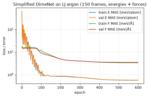
Let us plot the training curves for energy and force MAE over the epochs

ax = plot_training_curves(history)
ax.set_title("Simplified DimeNet on LJ argon (150 frames, energies + forces)")
ax.figure.tight_layout()

We can now create a parity plot for the predicted forces vs. the reference forces.

model.eval()
_, F_val = energy_and_forces(model, *val_batch[:6], len(val_batch[6]))
F_pred = F_val.detach().cpu().numpy().ravel() * 1e3
F_true = val_batch[7].cpu().numpy().ravel() * 1e3

fig, ax = plt.subplots(figsize=(4.6, 4.6))
lim = np.abs(F_true).max() * 1.1
ax.plot([-lim, lim], [-lim, lim], "--", color="gray", lw=1, label="parity")
ax.scatter(F_true, F_pred, s=8, alpha=0.4, color="C0", edgecolors="none")
ax.set_xlim(-lim, lim); ax.set_ylim(-lim, lim); ax.set_aspect("equal")
ax.set_xlabel("reference force component [meV/Å]")
ax.set_ylabel("predicted force component [meV/Å]")
ax.set_title("Validation forces: predicted vs. reference")
ax.legend(); ax.grid(True, alpha=0.3); fig.tight_layout()

e_mae, f_mae = eval_mae(model, val_batch)
schnet_07a = {"E": 0.097, "F": 0.678}
print(f"{'model':>26} | {'val E MAE [meV/atom]':>21} | {'val F MAE [meV/Å]':>18}")
print(f"{'SchNet (Lesson 07a)':>26} | {schnet_07a['E']:>21.3f} | {schnet_07a['F']:>18.3f}")
print(f"{'SimpleDimeNet (Lesson 07b)':>26} | {e_mae:>21.3f} | {f_mae:>18.3f}")

                     model |  val E MAE [meV/atom] |  val F MAE [meV/Å]
       SchNet (Lesson 07a) |                 0.097 |              0.678
SimpleDimeNet (Lesson 07b) |                 0.570 |              3.463

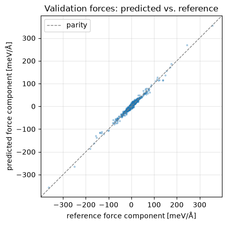
Both models reach sub-meV energy accuracy, and the angular model brings no decisive advantage here, exactly as argued above: as a pair potential, the LJ expression can describe the interactions within the argon dataset and distances already contain everything required to allow the dGNN models to learn the underlying physics. Keep this experiment in mind as a control: the architectural sophistication only pays off when the data and the target property contain the corresponding physics. On angle-dependent systems (molecules, covalent solids, the degenerate pairs of Section 1) the picture reverses dramatically. This is our motivation for another round of trainings on a dataset with genuine angular information in Lesson 07c.

13.4. Numerical verification of invariance

The distances and angles are both invariant under \(E(3)\) (including parity: \(\cos\alpha\) is a ratio of dot products, both of which are parity-even). Therefore, the energy must be a 0e scalar and the forces 1o vectors, with the graph and triplets rebuilt after each transform. (As in Lesson 07a, the harness’s force check is limited to \(\sim 10^{-7}\) by e3nn’s D_from_matrix; the direct check against \(R\) itself confirms exactness in float64.)

# Check the equivariance of the model on a single frame
model64 = copy.deepcopy(model).double().cpu().eval()

# Take the first validation frame as a test case
pos_test = val_frames[0]["pos"].clone()

# Create dummy species and batch tensors for the test frame
z_test = torch.zeros(n_atoms, dtype=torch.long)
b_test = torch.zeros(n_atoms, dtype=torch.long)

# Build the graph and triplets for the test frame
def graph_of(pos):
    ei = radius_graph(pos.detach() if pos.requires_grad else pos, R_CUT)
    return (ei, *find_triplets(ei))

# Define energy function
def energy_fn(pos):
    ei, ta, tb = graph_of(pos)
    return model64(pos, z_test, ei, ta, tb, b_test, 1).reshape(1)

# Define force function
def force_fn(pos):
    ei, ta, tb = graph_of(pos)
    _, F = energy_and_forces(model64, pos, z_test, ei, ta, tb, b_test, 1)
    return F

# Check the equivariance of the energy and forces under rotations and translations
print("energy  E(RX + t) = E(X):")
assert_model_equivariant(energy_fn, pos_test, "0e", tol=1e-12)
print("forces  F(RX + t) = R F(X)  (harness):")
assert_model_equivariant(force_fn, pos_test, "1o", tol=1e-6)

# Check the forces for exact covariance under random rotations and translations
err, F_ref = 0.0, force_fn(pos_test)
for _ in range(5):
    R = o3.rand_matrix(dtype=torch.float64)
    # Improper rotations: parity too
    if torch.rand(()) < 0.5: R = -R
    t = torch.randn(3, dtype=torch.float64)
    err = max(err, (force_fn(pos_test @ R.T + t) - F_ref @ R.T).abs().max().item())

assert err < 1e-12, err
print(f"forces exactly covariant: max |F(RX+t) - R F(X)| = {err:.3e}  (float64)")

energy  E(RX + t) = E(X):
equivariant!  (max error 9.021e-17 over random O(3) + translations elements)
forces  F(RX + t) = R F(X)  (harness):
equivariant!  (max error 1.073e-08 over random O(3) + translations elements)
forces exactly covariant: max |F(RX+t) - R F(X)| = 4.406e-16  (float64)

13.5. What do triplets cost? \(O(Nk^2)\) vs. \(O(Nk)\)

Let \(k\) be the average number of neighbors within the cutoff. Per structure:

• Pairwise message passing (Lesson 07a): one message per directed edge will result in \(O(Nk)\) messages.

• Directional message passing (Lesson 07b): one interaction per edge pair sharing a vertex, \(\sum_j \deg(j)\big(\deg(j) - 1\big) \approx O(Nk^2)\) triplets.

Our training batch above makes this estimation concrete: Since our LJ gas is dilute (\(k \approx 3.4\)), with \(N = 1200\) atoms we had \(\approx 4000\) edges but \(\approx 10^4\) triplets. In a liquid or solid with \(k \approx 30-60\), the \(k^2\) factor is a 1-2 order of magnitude overhead, and extending the same logic to torsions/dihedrals (GemNet-style quadruplets) costs \(O(Nk^3)\). DimeNet++’s Hadamard trick cuts the constant \(\approx\) 8×, but the scaling stands.

13.6. Moving forward

Instead of enumerating triplets of invariant scalars, we can let each message itself carry directional content: spherical-harmonic features of order \(l > 0\) that rotate with the structure (as we saw in Lessons 02b-06a). A tensor product of two \(l = 1\) features already encodes angular correlations, so equivariant networks capture 3-body (and higher) geometry with only \(O(Nk)\) messages. That is precisely the design of NequIP model in Lessons 08a and 8b.

13.7. Summary

In this lesson we have learned:

• dGNNs are incomplete: the Pozdnyakov–Ceriotti \(\mathcal{A}^\pm\) pairs share every per-node distance multiset at any cutoff, yet are genuinely different: we built them, verified the distance/angle multisets, and showed a random dGNN yields identical energy predictions while our angular model can separate them.

• Directional message passing DimeNet, while embedding directed edges and using triplets with a joint basis in \((d_{kj}, \alpha^{(kj,ji)})\), stays invariant because distances and angles are invariant scalars.

• Physically motivated bases: DimeNet uses radial Bessel functions with a smooth envelope which is \(\mathcal{C}^2\) at the cutoff. DimeNet++ replaces the bilinear triplet layer with a Hadamard product and small MLPs making it 8× faster and \(\approx\) 10% more accurate on QM9 than DimeNet.

• On LJ argon the angular machinery buys little: The target is a pair potential whereas the angular features matter for covalent/directional systems and degenerate geometries.

• Triplets cost \(O(Nk^2)\) vs. \(O(Nk)\) for pairwise messages.

Next: Lesson 07c offers a dataset with genuine angular information, where the DimeNet-style model can shine. We compare its performance to that of SchNet and explain the reasons behind the observed differences.

13.8. Exercises

1. Near-degenerate structures (Difficulty: 🌶️🌶️🌶️): The pair \(\mathcal{A}^\pm\) built above is degenerate exactly: the two structures share the same distance multiset, so MiniDGNN returns identical energies to machine precision. Configurations encountered in practice (e.g., sampled by MD) will almost never be exactly degenerate. So, one might hope the problem is confined to a measure-zero set of geometries and can be ignored. Here, we test this hypothesis.

For each noise scale \(\epsilon \in \{10^{-3}, 10^{-2}, 10^{-1}\}\) Å, draw independent Gaussian displacements \(\delta^+, \delta^- \sim \mathcal{N}(0, \epsilon^2)\) for every coordinate and evaluate the same random, untrained dgnn (in float64) on the perturbed structures \(\mathcal{A}^+ + \delta^+\) and \(\mathcal{A}^- + \delta^-\). Average \(|\Delta E| = |E(\mathcal{A}^+ + \delta^+) - E(\mathcal{A}^- + \delta^-)|\) over about 20 noise draws per \(\epsilon\) and plot it against \(\epsilon\) on log–log axes. From that plot, answer the following questions:

• (a) What slope do you observe, and why?

• (b) The perturbed structures are still two genuinely different shapes: their angles, and hence in general their true energies, differ by an amount that does not shrink with \(\epsilon\). Explain why the result of (a) implies that a distance-only model has an irreducible error not only on the exact pair but throughout a finite neighborhood of configuration space around it, no matter how it is trained.

Solution

The following code generates the answer, reusing A_plus, A_minus and the random dgnn defined earlier in this lesson:

# Set the random seed for reproducibility
torch.manual_seed(0)

# List of noise scales to test
eps_list, mean_dE = [1e-3, 1e-2, 1e-1], []

# 
for eps in eps_list:
    dE = []
    # 20 independent noise draws
    for _ in range(20):

        # Add Gaussian noise to the positions of A_plus and A_minus
        Ep = dgnn(A_plus  + eps * torch.randn_like(A_plus)).item()
        Em = dgnn(A_minus + eps * torch.randn_like(A_minus)).item()
        
        # Compute the absolute energy difference and store it
        dE.append(abs(Ep - Em))
    
    # Compute the mean of the absolute energy differences for this noise scale
    mean_dE.append(np.mean(dE))
    print(f"eps = {eps:.0e} Å   mean |E(A+) - E(A-)| = {mean_dE[-1]:.3e}")

# Fit a line to the log-log data to find the slope
slope = np.polyfit(np.log(eps_list), np.log(mean_dE), 1)[0]
print(f"log-log slope = {slope:.2f}   (1.0 = linear growth)")

# Plot the results on a log-log scale
fig, ax = plt.subplots(figsize=(4.5, 3.4))
ax.loglog(eps_list, mean_dE, "o-", label=r"mean $|\Delta E|$ (20 draws)")
ax.loglog(eps_list, np.array(eps_list) * mean_dE[0] / eps_list[0], "--",
          color="gray", label=r"$\propto \epsilon$ (slope 1)")
ax.set_xlabel(r"noise scale $\epsilon$ [Å]")
ax.set_ylabel(r"$|E(\mathcal{A}^+ + \delta^+) - E(\mathcal{A}^- + \delta^-)|$")
ax.set_title("dGNN on a near-degenerate pair")
ax.legend()
ax.grid(True, alpha=0.3, which="both")
fig.tight_layout()

(a) The slope is \(\approx 1\), i.e., \(|\Delta E|\) grows linearly with \(\epsilon\). The network output \(E(X)\) is a smooth function of the positions, and at \(\epsilon = 0\) the two outputs coincide exactly. A first-order Taylor expansion around the unperturbed pair therefore gives \(\Delta E \approx \nabla E(\mathcal{A}^+)\!\cdot\!\delta^+ - \nabla E(\mathcal{A}^-)\!\cdot\!\delta^- = O(\epsilon)\): the difference starts from zero and can only grow as fast as the displacement.

(b) Let \(\Delta E_\mathrm{true}\) be the (finite, \(\epsilon\)-independent) true energy difference between the two perturbed structures, and let \(C\) bound the gradient of the model. By (a), the model can separate the two by at most \(\approx C\epsilon\). Whenever \(C\epsilon \ll \Delta E_\mathrm{true}\), at least one of the two predictions must be wrong by \(\approx \Delta E_\mathrm{true}/2\). Since this holds for every pair of configurations within a distance \(\approx \Delta E_\mathrm{true}/C\) of the degenerate pair, the error floor covers a region of finite volume in configuration space, not just the two exact geometries. No amount of training can remove it, because it follows from smoothness plus the fact that the model depends on distances only. Adding angular information (such as DimeNet) breaks the degeneracy already at \(\epsilon = 0\) and thereby removes the floor.

2. Ablate the angles (Difficulty: 🌶️): Set n_ang=1 in SimpleDimeNet (the angular basis reduces to the constant \(T_0 = 1\), so triplet aggregation still happens but carries no angular resolution) and re-run the \(\mathcal{A}^\pm\) pair counterexample check and the training. What changes?

Solution

With n_ang=1, the SimpleDimeNet model uses the distances and their embeddings, \(e_{\mathrm{RBF}}(d_{kj})\) only. As such, the model becomes a (fancier) dGNN: the \(\mathcal{A}^\pm\) pair counterexample energies coincide again, while the LJ validation errors stay essentially unchanged (as describing the LJ potential requires no angular information). This isolates where the extra expressive power comes from: the \(m \geq 1\) angular basis functions.

3. Measure the scaling (Difficulty: 🌶️🌶️): Generate LJ frames for argon with n_atoms \(\in\) \(\{8, 16, 32, 64\}\) while scaling the box as box \(= 7.0\,(N/8)^{1/3}\) Å so that the density stays constant. Count the number of directed edges and triplets at \(r_\mathrm{cut} = 6\) Å using radius_graph and find_triplets. Plot both counts vs. \(N\) on a log–log scale and fit the slopes. Do they match the expected costs of \(O(Nk)\) for edges and \(O(Nk^2)\) for triplets? Check whether \(k\) (the average number of neighbors per atom, \(\mathrm{edges}/N\)) is actually constant across your scans before interpreting the slopes. Then, take one 64-atom frame and sweep the cutoff \(r_\mathrm{cut} \in \{4, 6, 8\}\) Å at a fixed geometry: How do the two counts grow with \(k\) now?

Solution

# Count edges and triplets in a single frame
def count_edges_triplets(pos, r_cut):
    ei = radius_graph(pos, r_cut)
    trip_a, _ = find_triplets(ei)
    return ei.shape[1], len(trip_a)

# (i) Constant density: box grows as N^(1/3)
Ns, n_edges, n_trips, ks = [8, 16, 32, 64], [], [], []
for n in Ns:
    # Scale the box to keep density constant
    box = 7.0 * (n / 8) ** (1 / 3)

    # Generate a small LJ argon dataset
    frs = make_lj_argon_dataset(n_frames=3, n_atoms=n, box=box, seed=0)

    # Count edges and triplets for each frame
    E_, T_ = zip(*[count_edges_triplets(f["pos"], 6.0) for f in frs])

    # Compute the mean counts across frames
    n_edges.append(np.mean(E_))
    n_trips.append(np.mean(T_))
    ks.append(n_edges[-1] / n)
    print(f"N={n:3d}  box={box:5.2f} Å   edges={n_edges[-1]:7.1f}   "
          f"triplets={n_trips[-1]:8.1f}   k={ks[-1]:.2f}")

# Fit log-log slopes vs N
s_e = np.polyfit(np.log(Ns), np.log(n_edges), 1)[0]
s_t = np.polyfit(np.log(Ns), np.log(n_trips), 1)[0]
print(f"log-log slopes vs N:  edges {s_e:.2f},  triplets {s_t:.2f}")

# Plot the counts vs N on log-log axes
fig, ax = plt.subplots(figsize=(4.6, 3.4))
ax.loglog(Ns, n_edges, "o-", label=f"edges (slope {s_e:.2f})")
ax.loglog(Ns, n_trips, "s-", label=f"triplets (slope {s_t:.2f})")
ax.set_xlabel("number of atoms $N$")
ax.set_ylabel("count")
ax.set_title(r"Edge vs. triplet count at $r_\mathrm{cut} = 6$ Å")
ax.legend()
ax.grid(True, alpha=0.3, which="both")
fig.tight_layout()

# (ii) Growing k: one 64-atom frame, increasing cutoff
# Create a single frame of 64 atoms
pos64 = make_lj_argon_dataset(n_frames=1, n_atoms=64, box=14.0, seed=0)[0]["pos"]

# Sweep the cutoff and count edges and triplets
for r in [4.0, 6.0, 8.0]:
    E_, T_ = count_edges_triplets(pos64, r)
    print(f"r_cut={r:4.1f} Å   k={E_/64:5.2f}   edges={E_:5d}   "
          f"triplets={T_:6d}   triplets/edges={T_/E_:6.2f}")

(i) The counts follow \(|\text{edges}| \approx Nk\) and \(|\text{triplets}| \approx Nk(k-1)\) but the fitted slopes come out above 1 (\(s_\text{edges} \approx 1.4\) and \(s_\text{triplets} \approx 1.9\)). The code generates a table which shows why the discrepancy appears: \(k\) does not remain constant across this scan (\(k \approx 3.8 \to 9.5\)). Our clusters are small and non-periodic. Therefore, at \(r_\mathrm{cut} = 6\) Å, most atoms sit near the cluster “surface” and see fewer neighbors than a bulk atom would. Meanwhile, \(k\) is still climbing toward its bulk value as \(N\) grows. The scaling laws still hold in the form \(\log(\text{edges}) = \log N + \log k\) and \(\log(\text{triplets}) \approx \log N + 2\log k\), which predicts \(s_\text{triplets} \approx 2\,s_\text{edges} - 1\), which is satisfied by the fitted slopes. In a truly bulk (periodic) system \(k\) would be constant and both slopes would flatten to 1.

(ii) At fixed geometry, the cutoff sweep isolates the \(k\)-dependence: raising \(r_\mathrm{cut}\) from 4 to 8 Å grows \(k\) from about 3 to 19. Meanwhile, as the edge count grows \(\propto k\), the triplet count grows \(\propto k^2\). This can be observed directly via calculating the triplets/edges ratio, which is
\(\approx k - 1\) (slightly above, because \(k\) varies from atom to atom). This is the \(O(Nk^2)\) cost of directional message passing: it is the neighborhood size, not the system size, that makes the triplets expensive. This cost is one of the motivations behind introducing equivariant features in Part IV which can recover the angular information at \(O(Nk)\) cost.

13.9. References

• Pozdnyakov & Ceriotti, Incompleteness of graph neural networks for point clouds in three dimensions arXiv.2201.07136 2022

• Gasteiger et al., Directional Message Passing for Molecular Graphs arXiv.2003.03123 (2020)

• Gasteiger et al., Fast and Uncertainty-Aware Directional Message Passing for Non-Equilibrium Molecules arXiv.2011.14115 (2022)