17. Lesson 08c: Training NequIP and the rMD17 Rematch

What you will learn

• Train the SimpleNequIP architecture of Lesson 08b with a joint energy + force loss, and analyze its learning curves and force parity plot.

• Test for equivariance after the training to confirm that gradient descent cannot damage a symmetry that is built into the architecture.

• Run the same model against the Lesson 07’s SchNet and DimeNet baselines on rMD17 aspirin.

• Export the trained checkpoint to artifacts/ for Lesson 11 to enable running a molecular dynamics simulation with it.

Prerequisites:

• Lesson 08b: the SimpleNequIP implementation and the generated module, artifacts/nequip_model.py, which this lesson imports,

• Lesson 08a: the loss function and the scale/shift initialization,

• Lesson 07a, 07b and 07c: SchNet, DimeNet++, and the argon/aspirin protocol whose results we compare against here.

Note: The architecture itself is not rebuilt here. Lesson 08b packaged it as a module (artifacts/nequip_model.py), and this lesson imports it as one. Run Lesson 08b first if the nequip_model.py file is not in the notebooks/artifacts/ for any reason.

import sys
sys.path.insert(0, "..")    # Make course_utils importable
sys.path.insert(0, "")      # Make ./artifacts importable

import copy
import pathlib
import time

import matplotlib.pyplot as plt
import numpy as np
import torch
from e3nn import o3

from course_utils.data import make_lj_argon_dataset, radius_graph, train_val_split, load_rmd17
from course_utils.plotting import plot_training_curves

# The architecture, imported from the module Lesson 08b generated
from artifacts.nequip_model import SimpleNequIP, energy_and_forces


torch.manual_seed(0)
device = "cuda" if torch.cuda.is_available() else "cpu"
# dtype strategy: float32 (default) for training speed; equivariance checks use float64 copies.
print(f"torch {torch.__version__} | device: {device}")

torch 2.7.1+cu126 | device: cuda

17.1. The dataset and the model

In this lesson, we reuse our previous setup in Lesson 08b exactly: the same 200-frame Lennard-Jones argon trajectory (course_utils.data.make_lj_argon_dataset, \(\varepsilon = 0.0104\) eV, \(\sigma = 3.4\) Å, 8 atoms), the same deterministic 150 train / 50 validation split, the same \(r_c = 6\) Å, and the same average neighbor count \(\bar N\) that normalizes the convolution. Because both the generator and the split are seeded, the numbers below match the ones 08b printed.

# The same data as Lesson 08b: seeded generator, seeded split
frames = make_lj_argon_dataset(n_frames=200, n_atoms=8, seed=0)
train_frames, val_frames = train_val_split(frames, val_fraction=0.25, seed=0)
n_atoms = frames[0]["pos"].shape[0]
r_cut = 6.0

# Average number of neighbors over the training set: the convolution's 1/sqrt(N_bar)
avg_num_neighbors = float(np.mean(
    [radius_graph(f["pos"], r_cut).shape[1] / n_atoms for f in train_frames]))

# A fixed reference geometry, reused for the post-training symmetry re-check
# float64 (8, 3)
pos0 = frames[0]["pos"].clone()
edges0 = radius_graph(pos0, r_cut)

# Print some information about the data
print(f"{len(train_frames)} train / {len(val_frames)} val frames, {n_atoms} atoms each")
print(f"average number of neighbors within r_c = {r_cut} Å:  {avg_num_neighbors:.2f}")
print(f"imported SimpleNequIP from {SimpleNequIP.__module__}")

150 train / 50 val frames, 8 atoms each
average number of neighbors within r_c = 6.0 Å:  3.37
imported SimpleNequIP from artifacts.nequip_model

/D4/sina/PROJECTS/e3nn-course/.venv/lib/python3.13/site-packages/ase/md/langevin.py:102: FutureWarning: The implementation of `fixcm=True` in `Langevin` does not strictly sample the correct NVT distributions. The deviations are typically small for large systems but can be more pronounced for small systems. Use `fixcm=False` together with `ase.constraints.FixCom`. `fixcm` is deprecated since ASE 3.28.0 and will be removed in a future release.
  warnings.warn(msg, FutureWarning)

17.2. Training with the joint energy + force loss

The NequIP manuscript trains the model with a loss function based on a weighted sum of energy and atomic forces:

(1)\[\mathcal{L} \;=\; \lambda_E\, \big\|\hat E - E\big\|^2 \;+\; \frac{\lambda_F}{3N} \sum_{i=1}^{N} \sum_{\alpha=1}^{3} \bigg\| -\frac{\partial \hat E}{\partial r_{i,\alpha}} - F_{i,\alpha} \bigg\|^2, \]

where \(N\) is the number of atoms, \(E\) is the reference total energy, \(\hat E\) is the predicted total energy, and \(F_{i,\alpha}\) denotes the reference force components. The authors have found that a suitable default choice for the relative weighting of energies to forces is 1 to \(N^2_\mathrm{atoms}\), which for our argon dataset translates to \(\lambda_E = 1\), and \(\lambda_F = 8^2 = 64\). The \(N\)-scaling makes the loss size-invariant as for each system, the energy is one global label, and the forces are \(3N\) local ones.

Here, instead of rescaling the target energies and forces, we initialize the model’s energy_shift to the mean per-atom training energy and set the energy_scale to the root-mean-square (RMS) of training force components which is the single-species analogue of the NequIP manuscript’s scale and shift parameters.

The datasets we have chosen for this course are often tiny. So, we train our models using full-batches of samples: all 150 training frames are packed into one disconnected graph (per-frame batch indices route each atomic energy to its own sum).

Time to turn everything we detailed above into code and train the model! First, let us implement a collate function that packs a list of frames into one disconnected graph

def collate(frame_list, dtype=torch.float32):
    '''Pack frames into one disconnected graph: positions, offset edges, graph
    ids, targets.'''
    
    # Concatenate positions, forces, and energies into single tensors
    pos = torch.cat([f["pos"] for f in frame_list]).to(dtype)
    F = torch.cat([f["forces"] for f in frame_list]).to(dtype)
    E = torch.tensor([f["energy"] for f in frame_list], dtype=dtype)
    
    # Build the edge index and batch vector for the disconnected graph
    edges, batch, offset = [], [], 0
    for k, f in enumerate(frame_list):
        
        # The radius_graph function returns a 2xE tensor of edges, where E is the number of edges.
        edges.append(radius_graph(f["pos"], r_cut) + offset)
        
        # The batch vector indicates which frame each atom belongs to. It has
        # the same length as the number of atoms in the concatenated positions
        # tensor.
        batch.append(torch.full((f["pos"].shape[0],), k, dtype=torch.long))
        
        # The offset is used to adjust the edge indices for the next frame.
        # Since we are concatenating the positions of all frames, the edge
        # indices for each frame need to be shifted by the number of atoms in
        # the previous frames.
        offset += f["pos"].shape[0]
        
    # Return the concatenated positions, edges, batch vector, energies, and forces.
    return pos, torch.cat(edges, dim=1), torch.cat(batch), E, F

# Collate the training and validation frames into disconnected graphs and move
# them to the device (CPU or GPU).
pos_tr, edges_tr, batch_tr, E_tr, F_tr = [x.to(device) for x in collate(train_frames)]
pos_va, edges_va, batch_va, E_va, F_va = [x.to(device) for x in collate(val_frames)]

# Print the number of atoms, edges, and frames in the training graph. The number
# of atoms is the number of rows in the positions tensor, the number of edges is
# the number of columns in the edges tensor, and the number of frames is one
# more than the maximum value in the batch vector (since batch indices start at
# 0).
print(f"train graph: {pos_tr.shape[0]} atoms, {edges_tr.shape[1]} edges, {int(batch_tr.max())+1} frames")

train graph: 1200 atoms, 4044 edges, 150 frames

Now, we initialize the model, the optimizer and the learning rate scheduler

# Initialize the model
model = SimpleNequIP(r_cut=r_cut, avg_num_neighbors=avg_num_neighbors).to(device)

# Initialize scale/shift
with torch.no_grad():
    model.energy_shift.fill_((E_tr / n_atoms).mean().item())     # mean per-atom energy
    model.energy_scale.fill_(F_tr.pow(2).mean().sqrt().item())   # force-component RMS
print(f"parameters: {sum(p.numel() for p in model.parameters()):,}")
print(f"energy_shift = {model.energy_shift.item():+.5f} eV/atom, "
      f"energy_scale = {model.energy_scale.item():.5f} eV")

# The lambda values for the energy and force loss terms
lam_E, lam_F = 1.0, float(n_atoms**2)

# Instantiate the optimizer and learning rate scheduler
optimizer = torch.optim.Adam(model.parameters(), lr=5e-3)
scheduler = torch.optim.lr_scheduler.StepLR(optimizer, step_size=150, gamma=0.5)

parameters: 70,762
energy_shift = -0.00945 eV/atom, energy_scale = 0.03238 eV

The next step is to implement the training loop

# Set the number of epochs 
n_epochs = 400

# Set up the training loop
history = {"train loss": [], "val E MAE [meV]": [], "val F MAE [meV/Å]": []}
t0 = time.time()
for epoch in range(n_epochs):
    # Put the model in training mode
    model.train()
    
    # Zero the gradients of the optimizer to prevent accumulation from previous steps
    optimizer.zero_grad()
    
    # Compute the predicted energies and forces for the training data using the model
    E_hat, F_hat = energy_and_forces(model, pos_tr.clone(), edges_tr, batch=batch_tr)
    
    # Using .mean() over force components realizes (1/3N) \sum_i \sum_\alpha; frames are averaged.
    loss = lam_E * ((E_hat - E_tr) ** 2).mean() + lam_F * ((F_hat - F_tr) ** 2).mean()
    
    # Backpropagate the loss to compute gradients
    loss.backward()
    
    # Update the model parameters using the optimizer
    optimizer.step()
    
    # Update the learning rate according to the scheduler
    scheduler.step()

    # Evaluate the model on the validation set
    model.eval()
    E_hv, F_hv = energy_and_forces(model, pos_va.clone(), edges_va, batch=batch_va)
    history["train loss"].append(loss.item())
    history["val E MAE [meV]"].append(1000 * (E_hv - E_va).abs().mean().item())
    history["val F MAE [meV/Å]"].append(1000 * (F_hv - F_va).abs().mean().item())
    
    # Print training progress every 50 epochs and at the last epoch
    if epoch % 50 == 0 or epoch == n_epochs - 1:
        print(f"epoch {epoch:3d} | loss {loss.item():.5f} | "
              f"val E MAE {history['val E MAE [meV]'][-1]:7.2f} meV | "
              f"val F MAE {history['val F MAE [meV/Å]'][-1]:6.2f} meV/Å | {time.time()-t0:5.1f} s")

# Print the total training time
print(f"total training time: {time.time() - t0:.1f} s on {device}")

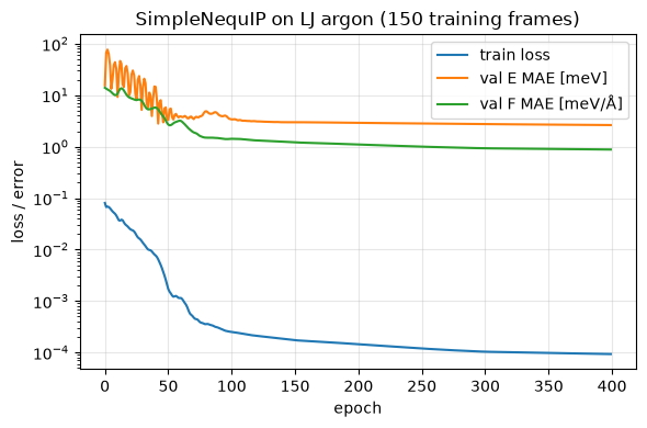
epoch   0 | loss 0.08062 | val E MAE   15.55 meV | val F MAE  14.00 meV/Å |   1.5 s
epoch  50 | loss 0.00170 | val E MAE    3.30 meV | val F MAE   2.69 meV/Å |  10.9 s
epoch 100 | loss 0.00025 | val E MAE    3.39 meV | val F MAE   1.42 meV/Å |  19.6 s
epoch 150 | loss 0.00017 | val E MAE    2.99 meV | val F MAE   1.21 meV/Å |  28.3 s
epoch 200 | loss 0.00014 | val E MAE    2.91 meV | val F MAE   1.10 meV/Å |  37.0 s
epoch 250 | loss 0.00012 | val E MAE    2.82 meV | val F MAE   1.00 meV/Å |  45.7 s
epoch 300 | loss 0.00010 | val E MAE    2.74 meV | val F MAE   0.93 meV/Å |  54.4 s
epoch 350 | loss 0.00010 | val E MAE    2.69 meV | val F MAE   0.90 meV/Å |  63.1 s
epoch 399 | loss 0.00009 | val E MAE    2.63 meV | val F MAE   0.88 meV/Å |  71.6 s
total training time: 71.6 s on cuda

Having trained the model, we can now visualize the learning curves and the force parity plot. The learning curves show how the training loss and validation errors evolve over epochs

# Visualize the training curves
ax = plot_training_curves(history)
ax.set_title("SimpleNequIP on LJ argon (150 training frames)")
ax.figure.tight_layout()
plt.show()

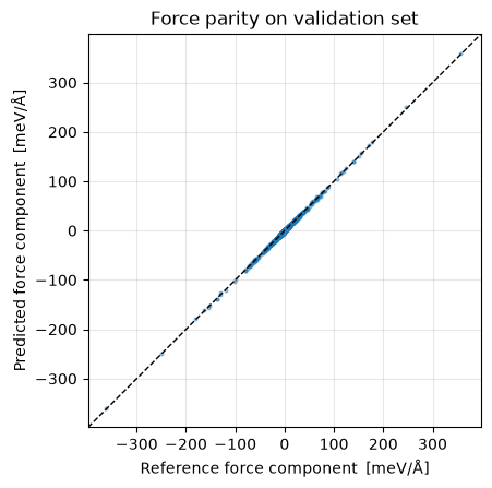
The force parity plot compares predicted forces against reference forces

# Set the model to evaluation mode
model.eval()

# Compute the predicted energies and forces for the validation data using the
# trained model
E_hv, F_hv = energy_and_forces(model, pos_va.clone(), edges_va, batch=batch_va)

# Compute the mean absolute error (MAE) for energy and force predictions on the
# validation set
mae_E = (E_hv - E_va).abs().mean().item()
mae_F = (F_hv - F_va).abs().mean().item()

# Print the validation energy and force MAE, scaled to meV and meV/Å
# respectively, along with the per-atom energy MAE
print(f"validation energy MAE: {1000 * mae_E:6.2f} meV  ({1000 * mae_E / n_atoms:.2f} meV/atom)")
print(f"validation force  MAE: {1000 * mae_F:6.2f} meV/Å  "
      f"(force RMS in data: {1000 * F_va.pow(2).mean().sqrt():.0f} meV/Å)")

# Create a force parity plot to visualize the agreement between predicted and
# reference forces
fig, ax = plt.subplots(figsize=(4.6, 4.6))
f_ref = F_va.cpu().numpy().ravel() * 1000
f_pred = F_hv.detach().cpu().numpy().ravel() * 1000
ax.scatter(f_ref, f_pred, s=4, alpha=0.4)
lim = np.abs(f_ref).max() * 1.1
ax.plot([-lim, lim], [-lim, lim], "k--", lw=1)
ax.set_xlim(-lim, lim); ax.set_ylim(-lim, lim)
ax.set_xlabel("Reference force component  [meV/Å]")
ax.set_ylabel("Predicted force component  [meV/Å]")
ax.set_title("Force parity on validation set")
ax.grid(alpha=0.3)
ax.set_aspect("equal")
fig.tight_layout()
plt.show()

validation energy MAE:   2.63 meV  (0.33 meV/atom)
validation force  MAE:   0.88 meV/Å  (force RMS in data: 32 meV/Å)

17.2.1. Equivariance survives the training

Symmetry in NequIP is built into the architecture and not learned. So, we expect that it remains untouched by the training. A quick re-check of the pre-trained weights in float64 gives us the verification we need

# Get the trained model in float64 and evaluate it on the reference geometry to
# check that equivariance is preserved after training
model64 = copy.deepcopy(model).cpu().to(torch.float64).eval()

# Compute the energy and forces for the reference geometry using the trained
# model
E0, F0 = energy_and_forces(model64, pos0.clone(), edges0)

# Improper random rotation
g = -o3.rand_matrix(dtype=torch.float64)

# Random translation
t = torch.randn(3, dtype=torch.float64)

# Compute the energy and forces for the transformed geometry using the trained
# model. The positions are transformed by the rotation and translation, and the
# edges are updated accordingly.
Eg, Fg = energy_and_forces(model64, pos0 @ g.T + t, edges0)

# Check that the energy and forces are equivariant under the transformation. The
# energy should be invariant, and the forces should transform according to the
# rotation matrix. The maximum absolute differences are printed to verify this.
print(f"Trained model:  |ΔE| = {(Eg - E0).abs().max():.2e},  "
      f"|ΔF| = {(Fg - F0 @ g.T).abs().max():.2e}   --> equivariance preserved")

Trained model:  |ΔE| = 5.03e-13,  |ΔF| = 5.46e-12   --> equivariance preserved

17.3. The rematch, part three: rMD17 aspirin

In Lessons 07b-07c, we conducted a set of controlled experiment, camparing the performance of SchNet against SimpleDimeNet, first on LJ argon dataset (where distances suffice), then on aspirin rMD17 dataset (where angles matter). The SimpleNequIP model promises angular expressiveness without the \(O(Nk^2)\) triplet enumeration.

We reuse Lesson 07c’s protocol for consistency: The official rMD17, split into (150 train / 50 validation frames), \(r_\mathrm{cut} = 5\) Å, mini-batches of 25 frames, Adam optimizer with cosine annealing, training for 600 epochs, the same loss with \(\rho = 1\), and the same per-atom mean shift of the energies. There is one exception: the learning rate is \(10^{-2}\) instead of \(3\times10^{-3}\).

We should also note that Lesson 07c’s hyperparameters were tuned for the invariant baselines, and the tensor-product network traied visibly slower there (it reached only \(\approx\) 121 meV/Å force MAE using the same budget). Each architecture adopted a learning rate that worked for its own case while every other knob remained identical. Nonethless, the aspirin dataset brought a new requirement for the models: three chemical elements (i.e., H, C, and O) compared to one (i.e., Ar). The species one-hot encoding (n_species=3) now does the real work, whereas for argon, the initial embedding was only a constant.

Let’s prepare the aspirin dataset and print some statistics about it

# Lesson 07c's data protocol: official rMD17 split 01, r_cut = 5 Å, per-atom mean shift
train_asp, val_asp, z_asp = load_rmd17("aspirin", n_train=150, n_val=50)

# Species mapping: {1:0, 6:1, 8:2}
species_map = {int(Z): s for s, Z in enumerate(torch.unique(z_asp).tolist())}

# Convert the atomic numbers in z_asp to species indices using the species_map.
# This creates a tensor of species indices corresponding to each atom in the
# aspirin molecule.
species_asp = torch.tensor([species_map[int(Z)] for Z in z_asp])

# Set the number of atoms and the cutoff radius for the aspirin dataset
n_atoms_asp, r_cut_asp = len(z_asp), 5.0

# Compute the per-atom mean energy shift for the aspirin dataset. This is used to
# normalize the energies during training.
eps_bar = np.mean([f["energy"] for f in train_asp]) / n_atoms_asp

# Define a collate function for the aspirin dataset that includes species
# indices and the per-atom mean shift. This function takes a list of frames and
# returns the concatenated positions, edges, species indices, batch vector,
# energies (with mean shift), and forces.
def collate_asp(frame_list, dtype=torch.float32):
    '''collate() plus species indices and the per-atom mean shift, at r_cut = 5 Å.'''
    
    # Concatenate positions, forces, and energies into single tensors
    pos = torch.cat([f["pos"] for f in frame_list]).to(dtype)
    F = torch.cat([f["forces"] for f in frame_list]).to(dtype)
    E = torch.tensor([f["energy"] - len(f["pos"]) * eps_bar for f in frame_list], dtype=dtype)
    
    # Build the edge index, batch vector, and species indices for the
    # disconnected graph
    spec = species_asp.repeat(len(frame_list))
    edges, batch, offset = [], [], 0
    for k, f in enumerate(frame_list):
        edges.append(radius_graph(f["pos"], r_cut_asp) + offset)
        batch.append(torch.full((f["pos"].shape[0],), k, dtype=torch.long))
        offset += f["pos"].shape[0]
    
    # Return the concatenated positions, edges, species indices, batch vector,
    # energies, and forces.
    return pos, torch.cat(edges, dim=1), spec, torch.cat(batch), E, F

# Lesson 07c's training protocol: mini-batches of 25 frames
batches_asp = [tuple(x.to(device) for x in collate_asp(train_asp[i:i + 25]))
               for i in range(0, len(train_asp), 25)]

# Collate the validation frames into a single batch and move it to the device
val_batch_asp = tuple(x.to(device) for x in collate_asp(val_asp))

# Compute the average number of neighbors for the aspirin dataset using the
# radius_graph function. This is used to inform the model about the expected
# number of neighbors during training.
avg_nn_asp = float(np.mean([radius_graph(f["pos"], r_cut_asp).shape[1] / n_atoms_asp
                            for f in train_asp]))

# Print information about the aspirin dataset, including the number of atoms,
# the number of mini-batches, and the average number of neighbors.
print(f"Aspirin: {n_atoms_asp} atoms (H/C/O), {len(batches_asp)} mini-batches of 25 frames, "
      f"avg neighbors {avg_nn_asp:.1f}")

Aspirin: 21 atoms (H/C/O), 6 mini-batches of 25 frames, avg neighbors 14.4

With the aspirin dataset prepared, we can now proceed to train the SimpleNequIP model on this data.

# Set the random seed for reproducibility
torch.manual_seed(0)

# Initialize the SimpleNequIP model
model_asp = SimpleNequIP(r_cut=r_cut_asp, n_species=3,
                         avg_num_neighbors=avg_nn_asp).to(device)

# Initialize the energy shift and scale
# Same initialization recipe as for argon
with torch.no_grad():
    E_flat = torch.cat([b[4] for b in batches_asp])
    F_flat = torch.cat([b[5] for b in batches_asp])
    model_asp.energy_shift.fill_((E_flat / n_atoms_asp).mean().item())
    model_asp.energy_scale.fill_(F_flat.pow(2).mean().sqrt().item())

# Print the number of parameters in the model
print(f"parameters: {sum(p.numel() for p in model_asp.parameters()):,}")

# Set up the optimizer and learning rate scheduler
optimizer = torch.optim.Adam(model_asp.parameters(), lr=1e-2)
scheduler = torch.optim.lr_scheduler.CosineAnnealingLR(optimizer, T_max=600)

# Create the training loop
t0 = time.time()
for epoch in range(600):
    
    # Put the model in training mode
    model_asp.train()
    
    # Iterate over the mini-batches of the aspirin dataset
    for pos_b, edges_b, spec_b, batch_b, E_b, F_b in batches_asp:
        
        # Zero the gradients of the optimizer to prevent accumulation from
        # previous steps
        optimizer.zero_grad()
        
        # Compute the predicted energies and forces for the current mini-batch
        # using the model
        E_hat, F_hat = energy_and_forces(model_asp, pos_b.clone(), edges_b,
                                         species=spec_b, batch=batch_b)
        # Lesson 07c's loss with rho = 1
        loss = ((E_hat - E_b) ** 2).mean() + ((F_hat - F_b) ** 2).sum(dim=-1).mean()
        
        # Backpropagate the loss to compute gradients
        loss.backward()
        
        # Update the model parameters
        optimizer.step()
    
    # Update the learning rate according to the scheduler
    scheduler.step()
    
    # Evaluate the model on the validation set every 100 epochs and at the last
    # epoch
    if epoch % 100 == 0 or epoch == 599:
        
        # Put the model in evaluation mode
        model_asp.eval()
        
        # Compute the predicted energies and forces for the validation batch
        # using the trained model
        pos_v, edges_v, spec_v, batch_v, E_v, F_v = val_batch_asp
        E_hv, F_hv = energy_and_forces(model_asp, pos_v.clone(), edges_v,
                                       species=spec_v, batch=batch_v)
        
        # Print the epoch number, validation energy MAE, validation force MAE, and
        # elapsed time since the start of training
        print(f"epoch {epoch:3d} | val E MAE {1e3 * (E_hv - E_v).abs().mean().item() / n_atoms_asp:6.2f} meV/atom"
              f" | val F MAE {1e3 * (F_hv - F_v).abs().mean().item():7.2f} meV/Å"
              f" | {time.time() - t0:6.1f} s")
        
# Compute the total training time
dt_asp = time.time() - t0

# Print the total training time
print(f"total training time: {dt_asp:.0f} s on {device}")

parameters: 70,794
epoch   0 | val E MAE 115.22 meV/atom | val F MAE  925.34 meV/Å |    1.8 s
epoch 100 | val E MAE   6.71 meV/atom | val F MAE  160.10 meV/Å |   87.9 s
epoch 200 | val E MAE   7.03 meV/atom | val F MAE  112.39 meV/Å |  173.7 s
epoch 300 | val E MAE   4.11 meV/atom | val F MAE   96.04 meV/Å |  258.2 s
epoch 400 | val E MAE   1.65 meV/atom | val F MAE   88.75 meV/Å |  333.9 s
epoch 500 | val E MAE   1.52 meV/atom | val F MAE   85.86 meV/Å |  411.1 s
epoch 599 | val E MAE   1.51 meV/atom | val F MAE   85.29 meV/Å |  486.9 s
total training time: 487 s on cuda

The last step is to use the trained model to predict energies and forces on the validation set and compare them against the reference values from competitor models, SchNet and SimpleDimeNet.

# Put the model in evaluation mode
model_asp.eval()

# Compute the predicted energies and forces for the validation batch using the
# trained model
pos_v, edges_v, spec_v, batch_v, E_v, F_v = val_batch_asp
E_hv, F_hv = energy_and_forces(model_asp, pos_v.clone(), edges_v,
                               species=spec_v, batch=batch_v)
e_nequip = 1e3 * (E_hv - E_v).abs().mean().item() / n_atoms_asp
f_nequip = 1e3 * (F_hv - F_v).abs().mean().item()

# Lesson 07c's table, completed with a new third row for the SimpleNequIP model
print(f"{'val MAE, rMD17 aspirin':>24} | {'E [meV/atom]':>13} | {'F [meV/Å]':>10} | {'s/epoch':>8}")
print(f"{'SchNet (07c)':>24} | {2.35:>13.2f} | {128.61:>10.2f} | {0.09:>8.2f}")
print(f"{'SimpleDimeNet (07c)':>24} | {1.99:>13.2f} | {97.20:>10.2f} | {0.11:>8.2f}")
print(f"{'SimpleNequIP':>24} | {e_nequip:>13.2f} | {f_nequip:>10.2f} | {dt_asp / 600:>8.2f}")

# The same architecture on both datasets, each error against its dataset's force
# scale
f_rms_argon = 1e3 * F_va.pow(2).mean().sqrt().item()
f_rms_asp = 1e3 * F_v.pow(2).mean().sqrt().item()
print(f"\n{'SimpleNequIP, forces':>24} | {'MAE [meV/Å]':>11} | {'data RMS':>8} | relative")
print(f"{'LJ argon':>24} | {1e3 * mae_F:>11.2f} | {f_rms_argon:>8.0f} | {1e3 * mae_F / f_rms_argon:8.1%}")
print(f"{'rMD17 aspirin':>24} | {f_nequip:>11.2f} | {f_rms_asp:>8.0f} | {f_nequip / f_rms_asp:8.1%}")

  val MAE, rMD17 aspirin |  E [meV/atom] |  F [meV/Å] |  s/epoch
            SchNet (07c) |          2.35 |     128.61 |     0.09
     SimpleDimeNet (07c) |          1.99 |      97.20 |     0.11
            SimpleNequIP |          1.51 |      85.29 |     0.81

    SimpleNequIP, forces | MAE [meV/Å] | data RMS | relative
                LJ argon |        0.88 |       32 |     2.8%
           rMD17 aspirin |       85.29 |     1248 |     6.8%

17.3.1. Reading the result

• NequIP performs well within the course budget: With the species one-hot embeddings as the only architectural change, SimpleNequIP provides the best performance among the three models benchmarked on both energy and atomic forces at the same 150-frame rMD17 training budget: 1.51 meV/atom and 85 meV/Å against SimpleDimeNet’s 1.99 and 97 and SchNet’s 2.35 and 129. The \(l > 0\) features deliver the angular resolution that SimpleDimeNet captures using explicit triplets, and a little more, on pairwise messages alone.

• The cost of building messages is not trivial: At \(\approx\) 0.9 s/epoch against the SchNet’s baseline \(\approx\) 0.1 s, SimpleNequIP is the slowest model in the table. For NequIP, the message count scales as \(O(Nk)\) rather than \(O(Nk^2)\), but each message carries a tensor product, which costs far more than a scalar filter in SchNet. At 21 atoms, the constant factor win but the scaling argument pays off when the system is very large, e.g., at thousands of atoms. This cost is exactly the regime Lesson 09 chases using the Allegro model.

• Same machinery, a more difficult problem: Relative to each dataset’s force scale, the error is 2.8% on LJ argon and 6.8% on aspirin. Nothing about the model changed between the two experiments except n_species and the data pipeline: the architecture built for a pairwise toy potential moved to DFT-quality molecular forces by swapping the dataset.

17.4. Exporting the models for Lessons 11 and 13a

In Lesson 11, we wrap the pre-trained SimpleNequIP model as an ASE calculator and run molecular dynamics with it. We need two files in notebooks/artifacts/:

1. nequip_model.py, the model source module, already written by Lesson 08b, and

2. nequip_lj_argon.pt, the trained state_dict model artifact, plus the hyperparameter dict, written below.

We export the argon model for Lesson 11 because it compares the learned dynamics against the exact Lennard-Jones potential that generated the data, which is only possible for the toy system. We also export the aspirin model as nequip_aspirin.pt, which Lesson 13acoming soon opens up to ask what its features actually represent.

# Save the trained model and its hyperparameters to a checkpoint file in the
# artifacts directory. The checkpoint includes the model's state_dict,
# hyperparameters, and additional information about the dataset and validation
# errors.
art_dir = pathlib.Path("artifacts")
art_dir.mkdir(exist_ok=True)
checkpoint = {
    "state_dict": {k: v.cpu() for k, v in model.state_dict().items()},
    "hparams": model.hparams,
    "info": {"dataset": "make_lj_argon_dataset(n_frames=200, n_atoms=8, seed=0)",
             "val_energy_mae_eV": mae_E, "val_force_mae_eV_per_A": mae_F,
             "units": "eV, Å", "source": "08c_nequip_training.ipynb"},
}
torch.save(checkpoint, art_dir / "nequip_lj_argon.pt")
print(f"saved {art_dir / 'nequip_lj_argon.pt'} "
      f"({(art_dir / 'nequip_lj_argon.pt').stat().st_size / 1024:.0f} kB)")

saved artifacts/nequip_lj_argon.pt (315 kB)

# The aspirin model, for Lesson 13a's feature analysis. The species map is part of
# the artifact: without it, the one-hot embedding indices are meaningless.
checkpoint_asp = {
    "state_dict": {k: v.cpu() for k, v in model_asp.state_dict().items()},
    "hparams": model_asp.hparams,
    "info": {"dataset": "rMD17 aspirin, official split 01 (150 train / 50 val)",
             "species_map": species_map, "z": z_asp.tolist(),
             "val_energy_mae_meV_per_atom": e_nequip, "val_force_mae_meV_per_A": f_nequip,
             "units": "eV, Å", "source": "08c_nequip_training.ipynb"},
}
torch.save(checkpoint_asp, art_dir / "nequip_aspirin.pt")
print(f"saved {art_dir / 'nequip_aspirin.pt'} "
      f"({(art_dir / 'nequip_aspirin.pt').stat().st_size / 1024:.0f} kB)")

saved artifacts/nequip_aspirin.pt (316 kB)

17.4.1. Round-trip check

Similar to Lesson 08b, when we export a model artifact, we rebuild it again from its checkpoint which includes hyperparameters plus weights. Doing so, we want to make sure the loaded model artifact can reproduce the trained model’s predictions exactly, with no reference to a specific notebook state.

# Reload the model from the checkpoint
ckpt = torch.load(art_dir / "nequip_lj_argon.pt", weights_only=True)

# Recreate the model architecture using the hyperparameters stored in the
# checkpoint
model_reloaded = SimpleNequIP(**ckpt["hparams"])

# Load the state_dict from the checkpoint into the reloaded model
model_reloaded.load_state_dict(ckpt["state_dict"])

# Set the reloaded model to evaluation mode
model_reloaded.eval()


# Create a CPU copy of the trained model for comparison with the reloaded model. 
model_cpu = copy.deepcopy(model).cpu().eval()

# Get the positions of the first validation frame and convert them to float32
# for the radius_graph function. 
pos_check = val_frames[0]["pos"].to(torch.float32)

# Compute the edges for the first validation frame using the radius_graph
# function with the cutoff radius.
edges_check = radius_graph(pos_check, r_cut)

# Compute the energy and forces for the first validation frame using both the
# CPU copy of the trained model and the reloaded model.
E_a, F_a = energy_and_forces(model_cpu, pos_check.clone(), edges_check)
E_b, F_b = energy_and_forces(model_reloaded, pos_check.clone(), edges_check)

# Check that the energies and forces from both models are close to each other
# within a tolerance of 1e-7. This ensures that the reloaded model reproduces
# the predictions of the original trained model.
assert torch.allclose(E_a, E_b, atol=1e-7) and torch.allclose(F_a, F_b, atol=1e-7)
print(f"The reloaded model reproduces predictions:   (E = {E_a.item():+.5f} eV vs reference "
      f"{val_frames[0]['energy']:+.5f} eV)")

The reloaded model reproduces predictions:   (E = -0.08226 eV vs reference -0.08269 eV)

17.5. Summary

In this lesson, we have learned:

• How to train SimpleNequIP on 150 frames of LJ argon dataset with a joint loss of weighted combination of energy and force losses. The validation force MAE landed at a fraction of a meV/Å: about 2.8% of the force scale in the data in well under two minutes of GPU time.

• Equivariance survived the training: As it must! We have checked that the model can pass the symmetry test on random weights in Lesson 08b and on trained weights here with the same \(10^{-13}\) tolerance for equivariance.

• NequIP performs well on the aspirin rMD17 benchmark: Under Lesson 07c’s protocol (learning rate aside), SimpleNequIP reached 1.51 meV/atom and 85 meV/Å validation MAE: ahead of both SchNet (2.35, 128.6) and SimpleDimeNet (1.99, 97.2), with pairwise messages only, at the price of the slowest throughput in the table.

Next: Lesson 09acoming soon focuses on Allegro, which achieves equivariance without message passing: A feature that becomes important at large scales.

17.6. Exercises

1. Invariant baseline (Difficulty: 🌶️): Retrain the SimpleNequIP model which was trained on the LJ argon dataset, this time with l_max=0, while keeping every other setting and epoch budget the same. Compare the resulting model’s validation force MAE against the run in the main text. Then explain: why is the gap between the two models small on the LJ argon dataset, and why should it widen on the DFT data for molecules such as those in the aspirin rMD17 dataset?

Solution

Using the l_max=0 truncates the filter to 1x0e. So, the tensor product can only ever produce scalars. The 1o/1e channels of irreps_hidden are still allocated but stay identically zero, and the convolution collapses to SchNet-style scalar messages weighted by \(R(r)\). (Do not try to delete those channels by setting mul1=mul2=0: a Gate with nothing left to operate on raises a ValueError).

The difference gap is small for the LJ argon dataset because the energies depend only on the pair distances, which scalar messages can capture exactly. Distances alone are not sufficient to delineate the DFT interactions in molecules: bond angles, dihedrals and polarization require correlating the directions of several neighbors at once, which is what the \(l \ge 1\) features can bring into play (Lesson 08a). An invariant network must rebuild this spacial information indirectly, from overlapping distance patterns across several layers. For the aspirin dataset, the invariant baseline is handicapped by its inability to resolve the angular correlations in a single layer, and the gap widens between this basline and an equivariant model that uses the \(l \ge 1\) features to resolve the angular correlations directly.

2. Learned Bessel roots (Difficulty: 🌶️🌶️): The radial basis starts at the Bessel roots \(b\pi\) with \(b = 1, \dots, 8\), but basis.b_pi is trainable. Print model.basis.b_pi / torch.pi after training and see how far each frequency moved from its initial integer value. Then plot the trained basis over \(r \in [3, 6]\) Å, as Lesson 08b plots the initialized ones, and say which distance range the training sharpened. Note that the argon pairs cluster near the LJ minimum of \(2^{1/6}\sigma \approx 3.8\) Å.

Solution

from artifacts.nequip_model import BesselBasis

# Calculate the ratio of the learned Bessel roots to pi
ratio = (model.basis.b_pi / torch.pi).detach().cpu()

# Calculate the percentage shift of each learned Bessel root from its initial integer value
b = torch.arange(1, len(ratio) + 1)
shift = 100 * (ratio - b) / b

# Print the results
print("b_pi / pi :", " ".join(f"{v:6.3f}" for v in ratio))
print("shift [%] :", " ".join(f"{v:+6.1f}" for v in shift))

# Initialize a fresh Bessel basis for comparison
fresh = BesselBasis(r_cut, model.basis.n_basis)

# Create a range of r values for plotting
r = torch.linspace(0.5, r_cut, 400)

# Compute the trained and initial basis functions
with torch.no_grad():
    B_trained, B_initial = model.basis(r), fresh(r)

# Plot the trained and initial basis functions
fig, axes = plt.subplots(1, 2, figsize=(9.6, 3.4))
for k, color in ((0, "tab:blue"), (1, "tab:red")):
    axes[0].plot(r, B_initial[:, k], color=color, ls="--", lw=1.2, label=f"$b={k+1}$ initial")
    axes[0].plot(r, B_trained[:, k], color=color, lw=1.8, label=f"$b={k+1}$ trained")

# The LJ minimum
axes[0].axvline(2 ** (1 / 6) * 3.4, color="k", ls=":", lw=1.2)
axes[0].set_xlabel("pair distance $r$  [Å]")
axes[0].set_ylabel("$B_b(r)$")
axes[0].set_title("the two lowest frequencies")
axes[0].legend(fontsize=7)
axes[1].bar(b, shift, color="tab:blue")
axes[1].axhline(0, color="k", lw=0.8)
axes[1].set_xlabel("basis function $b$")
axes[1].set_ylabel(r"shift from $b\pi$  [%]")
axes[1].set_title("Where training moved the frequencies")
for ax in axes:
    ax.grid(alpha=0.3)
fig.tight_layout()
plt.show()

b_pi / pi :  1.059  1.931  3.017  3.940  4.994  5.981  7.014  8.075
shift [%] :   +5.9   -3.5   +0.6   -1.5   -0.1   -0.3   +0.2   +0.9

The basis barely moves. Every ratio stays within 6% of its initial integervalue, and the trained and initialized curves differ by at most 0.013 against a 0.35 peak which is about 3%. The physics-motivated initialization is already close to what the model wants to achieve, which is the argument for choosing it over a generic MLP of \(r\).

Most of the movement focus around the two lowest frequencies (\(+5.9\%\) for \(b = 1\), \(-3.5\%\) for \(b = 2\), against \(\leq 1.5\%\) for \(b \geq 3\); the latter being the ones with first-neighbor-shell structure). The node (where the value of the function is zero) of \(b = 2\) moves outward from 3.01 Å to 3.12 Å, toward the well minimum at \(2^{1/6}\sigma \approx 3.8\) Å, and \(b = 1\) gains a node at 5.67 Å. Faster functions oscillate beyond anything in the data and are untouched.

3. How much does the learning rate matter for NequIP’s performance? (Difficulty: 🌶️🌶️🌶️): The aspirin run in the text changes exactly one knob from Lesson 07c: the learning rate, which changes from \(3\times10^{-3}\) to \(10^{-2}\). Repeat the training experiment with a learning rate of \(3\times10^{-3}\) and \(5\times10^{-3}\) with everything else held fixed, and plot the three validation force-MAE curves on one axis. Is the slower model converging late, or converging to a worse solution? Before you answer, look at what CosineAnnealingLR(T_max=600) is doing to all three curves near epoch 600. Then, design an experiment that actually settles the question.

Solution

def run_at(lr, n_epochs=600):
    """The aspirin run of the main text, with the learning rate as a knob."""

    # Set the random seed for reproducibility
    torch.manual_seed(0)

    # Initialize the model and move it to the appropriate device
    m = SimpleNequIP(r_cut=r_cut_asp, n_species=3, avg_num_neighbors=avg_nn_asp).to(device)

    # Initialize the energy shift and scale based on the training batches
    with torch.no_grad():
        E_flat = torch.cat([b[4] for b in batches_asp])
        F_flat = torch.cat([b[5] for b in batches_asp])
        m.energy_shift.fill_((E_flat / n_atoms_asp).mean().item())
        m.energy_scale.fill_(F_flat.pow(2).mean().sqrt().item())

    # Set up the optimizer and learning rate scheduler
    opt = torch.optim.Adam(m.parameters(), lr=lr)
    sched = torch.optim.lr_scheduler.CosineAnnealingLR(opt, T_max=n_epochs)

    # Unpack the validation batch for later use
    pos_v, edges_v, spec_v, batch_v, E_v, F_v = val_batch_asp

    curve = []
    for epoch in range(n_epochs):
        m.train()
        for pos_b, edges_b, spec_b, batch_b, E_b, F_b in batches_asp:
            opt.zero_grad()
            E_hat, F_hat = energy_and_forces(m, pos_b.clone(), edges_b,
                                             species=spec_b, batch=batch_b)
            loss = ((E_hat - E_b) ** 2).mean() + ((F_hat - F_b) ** 2).sum(dim=-1).mean()
            loss.backward()
            opt.step()
        sched.step()

        m.eval()                                          # validate every epoch, for the curve
        _, F_hv = energy_and_forces(m, pos_v.clone(), edges_v, species=spec_v, batch=batch_v)
        curve.append(1e3 * (F_hv - F_v).abs().mean().item())
    return curve

# About 24 min on an A100 GPU
curves = {lr: run_at(lr) for lr in (1e-2, 5e-3, 3e-3)}

# Plot the three curves on one axis
fig, ax = plt.subplots(figsize=(6.4, 4.0))
for lr, curve in curves.items():
    ax.plot(curve, lw=1.5, label=f"lr = {lr:.0e}")
ax.set_yscale("log")
ax.set_xlabel("epoch")
ax.set_ylabel("validation force MAE  [meV/Å]")
ax.set_title("SimpleNequIP on rMD17 aspirin, one knob changed")
ax.grid(alpha=0.3)
ax.legend()
fig.tight_layout()
plt.show()

# Print the final validation force MAE and the gain over the last 50 epochs
for lr, curve in curves.items():
    print(f"lr {lr:.0e}: final {curve[-1]:7.2f} meV/Å"
          f" | gain over the last 50 epochs {curve[-50] - curve[-1]:.2f}")

lr 1e-02: final   85.28 meV/Å | gain over the last 50 epochs 0.07
lr 5e-03: final  104.51 meV/Å | gain over the last 50 epochs 0.07
lr 3e-03: final  121.23 meV/Å | gain over the last 50 epochs 0.07

The ordering holds at every epoch, not just the last one: 112 / 134 / 150 meV/Å at epoch 200, and 89 / 108 / 125 at epoch 400. The \(10^{-2}\) run reproduces the main text’s 85.28 meV/Å exactly.

But the flat tails do not indicate convergence: Each run gains 0.07 meV/Å over its last 50 epochs and nothing at all over their last 20. This is because the CosineAnnealingLR(T_max=600) drives the step size to zero on a schedule so that every run becomes flat at epoch 600 by construction. So, the tails cannot separate the two hypotheses. To address this issue, give the slower run the budget its own schedule implies instead:

# Run for another ~15 min
long = run_at(3e-3, n_epochs=1200)
print(f"lr 3e-03 at 1200 epochs: {long[-1]:.2f} meV/Å"
      f"  (600 epochs gave {curves[3e-3][-1]:.2f}; epoch 599 of this run: {long[599]:.2f})")

lr 3e-03 at 1200 epochs: 95.53 meV/Å  (600 epochs gave 121.23; epoch 599 of this run: 106.66)

Doubling the budget takes \(3\times10^{-3}\) from 121.23 to 95.53 meV/Å, closing 71% of the 35.9 meV/Å gap: mostly “converging late”, though 10.2 meV/Å survives at twice the cost.

At epoch 599, the longer run sits at 106.66 meV/Å while the shorter run, at the same epoch and the same learning rate, had been annealed down to 121.23: the schedule froze the model at a point it had not finished reaching. A learning rate and schedule tuned for one model family can handicap another at a fixed budget, and the handicap is indistinguishable from lower capacity unless you go looking, which is why this lesson flags its deviation from Lesson 07c’s protocol.

17.7. Reference

• Batzner et al., NequIP: E(3)-equivariant graph neural networks for data-efficient and accurate interatomic potentials Nat. Commun. 13 2453 (2022)