
12. Lesson 07a: SchNet and continuous-filter convolution#
What you will learn
Why distance-only features make a network invariant under rotations, translations and parity, and what the pros and cons of this design choice are.
The continuous-filter convolution (cfconv), SchNet’s core operation, and its filter-generating network.
How SchNet is assembled: atom-type embedding \(\to\) interaction blocks \(\to\) filter MLP \(\to\) element-wise product \(\to\) atom-wise layers \(\to\) atom-wise energy readout.
Why energy-conserving forces must come from \(\vec F_i = -\partial E / \partial \vec r_i\) (e.g., using autograd), and not from a separate force head.
Training on energies and forces with the standard weighted loss. We will verify the invariance of \(E\) and covariance of \(\vec F\) numerically.
Prerequisites:
Lesson 01a: Invariance vs. equivariance,
Lesson 05a: Atomistic graphs,
Lesson 05b: Radial bases and cutoffs.
import sys
sys.path.insert(0, "..")

import copy, time, warnings
import numpy as np
import torch
import torch.nn as nn
import matplotlib.pyplot as plt
from e3nn import o3

from course_utils.data import make_lj_argon_dataset, train_val_split, radius_graph
from course_utils.plotting import plot_training_curves
from course_utils.equivariance import assert_model_equivariant

warnings.filterwarnings("ignore", category=FutureWarning)  # ASE Langevin deprecation notice
torch.manual_seed(0)
np.random.seed(0)
device = "cuda" if torch.cuda.is_available() else "cpu"
print(f"device = {device}, torch {torch.__version__}")
device = cuda, torch 2.7.1+cu126
12.1. Why an invariant baseline?#
This lesson builds our first complete machine learning potential: a neural network that takes an atomistic configuration, nuclear charges and positions \(\{(Z_i, \vec r_i)\}_{i=1}^{n}\), and predicts its total energy \(\hat E\), from which the forces follow by differentiation. We begin by focusing on the SchNet ar chitecture, which we implement from scratch and train on frames of a molecular-dynamics trajectory of Lennard-Jones argon.
A potential energy is not an arbitrary function of the positions: rigidly translating, rotating, or reflecting an isolated system leaves its energy unchanged. Therefore, \(\hat E\) must be invariant under the Euclidean group \(E(3)\) operations.
In Parts I-II of this course, we have built the machinery for the general solution: networks whose internal features transform under rotations (rotational equivariance), and Part IV will use it to construct \(E(3)\)-equivariant potentials. Before that, we should study older, yet strong, alternatives: architectures that acquire invariance by restricting their inputs, throwing away all directional information and keeping only the interatomic distances.
To see why distances suffice, let us consider a rigid motion plus possible reflection acting on all positions, \(\vec r_i \mapsto R\,\vec r_i + \vec t\) with \(R \in O(3)\) (so \(R^\top R = I\), \(\det R = \pm 1\). The \(-1\) case corresponds to the parity/inversion operation) and \(\vec t \in \mathbb{R}^3\). The pairwise atomic distances remain unchanged under this transformation:
because \(\lVert R\vec v\rVert^2 = \vec v^\top R^\top R\, \vec v = \lVert\vec v\rVert^2\) for any orthogonal \(R\) including rotations and reflections. As such,
Any function of atom types and distances \(\{Z_i, d_{ij}\}\) is automatically invariant under the full Euclidean group, E(3), including parity. Consequently, the force (the gradient of the energy) becomes automatically equivariant.
This is the core design principle in SchNet: invariance is obtained by restricting the inputs, not by representation theory. An obvious drawback of distance-only models is that they are blind to angles and chirality within a cutoff: Lesson 07b shows that distance-only models such as SchNet are incomplete and cannot even distinguish certain environments, motivating Part IV of this course.
12.2. The continuous-filter convolution (cfconv)#
A discrete convolution slides a filter tensor over a grid of positions. In reality, atoms in a molecule or crystal often do not sit on a grid. So, SchNet replaces the filter tensor by a filter-generating function, \(W^l : \mathbb{R}^D \to \mathbb{R}^F\), evaluated at each relative position. With atom features, \(x_i^l \in \mathbb{R}^F\) at layer \(l\) (and feature dimension, \(F\)), the layer output can be expressed as:
where \(\odot\) is element-wise multiplication (compared to the convolution, which acts feature-wise and mixes the feature channels. This operation is assigned to separate atom-wise layers and will be discussed later in this lesson).
12.2.1. Restriction to distances#
In order to make the energy rotationally invariant, SchNet restricts the filter to depend only on the interatomic distance:
In our notation the sum runs over the neighbors of atom \(i\), i.e., \(j \in
\mathcal{N}(i)\) of a radius graph with cutoff \(r_\mathrm{cut}\). Recall the edge
convention from Lesson 05a: edge_index[0] = receiver \(i\), edge_index[1] =
sender \(j\), messages flow \(j \to i\).
12.2.2. Gaussian radial basis and the shifted softplus#
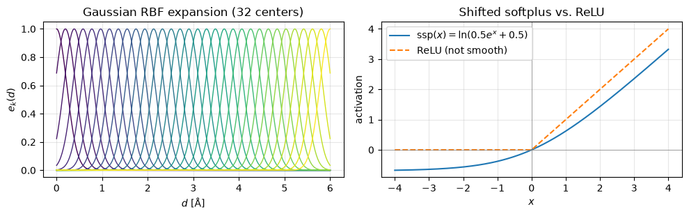
Feeding the raw scalar \(d_{ij}\) into an MLP makes the initial filters nearly linear in \(d\) and highly correlated, potentially leading to a training plateau. In order to overcome this issue, SchNet first expands the distance in Gaussian RBFs:
with centers, \(\mu_k\), placed on a regular grid in \(0\,\text{Å} \le \mu_k \le 30\,\text{Å}\) every \(0.1\) Å and \(\gamma = 10\,\text{Å}^{-2}\), chosen to cover all distances in the original training dataset.
We adapt the model training by using our own dataset of LJ-argon distances living below the cutoff value of \(r_\mathrm{cut} = 6\) Å. Here, we adopt 32 centers on \([0, r_\mathrm{cut}]\) and keep \(\gamma = 10\,\text{Å}^{-2}\).
Similar to SchNet, we use the shifted softplus for the nonlinearity:
which satisfies \(\mathrm{ssp}(0) = 0\) (helps convergence) and is \(C^\infty\)-smooth (i.e., infinitely differentiable). Smoothness matters because forces are the first derivatives of the network output, and training on forces back-propagates through the network, requiring the second derivatives. A network with a ReLU activation function has neither.
Let us implement the \(\mathrm{ssp}\) and the Gaussian RBF expansion in PyTorch.
# ssp(x) = ln(0.5 e^x + 0.5)
# = ln(1+e^x) - ln 2
def ssp(x):
    return nn.functional.softplus(x) - np.log(2.0)

# Gaussian RBF
class GaussianRBF(nn.Module):
    """e_k(d) = exp(-gamma (d - mu_k)^2)  on a regular grid of centers mu_k."""

    def __init__(self, r_cut: float, n_rbf: int = 32, gamma: float = 10.0):
        super().__init__()
        self.register_buffer("mu", torch.linspace(0.0, r_cut, n_rbf))
        self.gamma = gamma

    def forward(self, d):  # (E,) -> (E, n_rbf)
        return torch.exp(-self.gamma * (d.unsqueeze(-1) - self.mu) ** 2)

# Test the shifted softplus and Gaussian RBF
rbf = GaussianRBF(r_cut=6.0)
print("ssp(0) =", ssp(torch.tensor(0.0)).item())  # -> 0 by construction
print("RBF of 3 distances:", rbf(torch.tensor([3.0, 4.0, 5.0])).shape)
ssp(0) = 0.0
RBF of 3 distances: torch.Size([3, 32])
Having implemented the shifted softplus and Gaussian RBF, we can now visualize their behavior:
# Create a uniform grid of distances
d = torch.linspace(0, 6.0, 400)

# Evaluate the Gaussian RBF on the grid
# (400, 32)
E_k = rbf(d)

# Visualize the shifted softplus and Gaussian RBF
fig, (ax1, ax2) = plt.subplots(1, 2, figsize=(10, 3.2))
colors = plt.get_cmap("viridis")(np.linspace(0, 1, E_k.shape[1]))  # sequential: ordered centers
for k in range(E_k.shape[1]):
    ax1.plot(d, E_k[:, k], color=colors[k], lw=1)
ax1.set_xlabel(r"$d$ [Å]")
ax1.set_ylabel(r"$e_k(d)$")
ax1.set_title("Gaussian RBF expansion (32 centers)")
ax1.grid(True, alpha=0.3)

# Create a uniform grid of x values for the shifted softplus and ReLU
x = torch.linspace(-4, 4, 400)

# Visualize the shifted softplus and ReLU
ax2.plot(x, ssp(x), label=r"ssp$(x)=\ln(0.5e^x+0.5)$")
ax2.plot(x, nn.functional.relu(x), "--", label="ReLU (not smooth)")
ax2.axhline(0, color="gray", lw=0.5)
ax2.axvline(0, color="gray", lw=0.5)
ax2.set_xlabel(r"$x$")
ax2.set_ylabel("activation")
ax2.set_title("Shifted softplus vs. ReLU")
ax2.legend()
ax2.grid(True, alpha=0.3)
fig.tight_layout()
12.2.3. The filter-generating network#
The expanded distance is fed through two dense layers with (shifted) softplus activations to produce the filter values:
In this course, we slightly modify this network by multiplying the filter by a smooth cosine cutoff from Lesson 05b,
We perform this modification so that the resulting filters and the energy smoothly go to zero when a neighbor crosses the graph cutoff. Note that the original SchNet paper had no explicit cutoff (its RBF grid covered all distances in the specified range). Using the cutoff became a standard in the authors’ later SchNetPack implementation. Without the cutoff, atoms entering/leaving the radius graph would create small discontinuities in the potential energy surface as discussed in detail in Lesson 05b.
# Create a filter-generating network that takes distances and outputs filters
class FilterNet(nn.Module):
    '''W(d): distance -> R^F filter, RBF expansion + 2 dense layers + smooth cutoff.'''

    def __init__(self, n_features: int, r_cut: float, n_rbf: int = 32):
        super().__init__()

        # Gaussian RBF expansion of the distance
        self.rbf = GaussianRBF(r_cut, n_rbf)

        # Two dense layers
        self.dense1 = nn.Linear(n_rbf, n_features)
        self.dense2 = nn.Linear(n_features, n_features)

        # Cutoff distance for the smooth cosine cutoff
        self.r_cut = r_cut

    # (E,) -> (E, F)
    def forward(self, d):
        # Compute the filter values W(d) = ssp(W2 ssp(W1 e(d) + b1) + b2)
        W = ssp(self.dense2(ssp(self.dense1(self.rbf(d)))))

        # Smooth cutoff function f_cut(d) = 0.5 * (cos(pi d / r_cut) + 1)
        # Lesson 05b
        f_cut = 0.5 * (torch.cos(np.pi * d / self.r_cut) + 1.0)

        # Multiply the filter by the smooth cutoff so that it goes to zero
        # smoothly at r_cut
        return W * f_cut.unsqueeze(-1)

# Test the filter-generating network
W_test = FilterNet(n_features=64, r_cut=6.0)(torch.tensor([3.0, 5.999]))
print("filter shape:", W_test.shape, "| filter at d≈r_cut ~ 0:", W_test[1].abs().max().item())
filter shape: torch.Size([2, 64]) | filter at d≈r_cut ~ 0: 5.137263059395991e-09
12.3. The atom-wise layers#
The Atom-wise layers are dense layers applied to each atom’s feature vector separately, with weights shared across atoms:
They recombine feature channels (which the feature-wise cfconv deliberately does not) and keep the parameter count independent of the number of atoms.
12.4. The Interaction block#
Each block updates atoms through a residual connection
where the residual \(v_i^l\) is computed as: atom-wise layer \(\to\) cfconv \(\to\) atom-wise layer \(\to\) ssp \(\to\) atom-wise layer. In the code block below, each line is tagged with the component it implements.
class CFConv(nn.Module):
    '''Continuous-filter convolution:  x_i' = sum_{j in N(i)} x_j \\odot W(d_ij).'''

    def __init__(self, n_features: int, r_cut: float):
        super().__init__()
        # Create a filter-generating network that takes distances and outputs filters
        self.filter_net = FilterNet(n_features, r_cut)

    def forward(self, x, edge_index, d):
        # Receiver i, sender j  (05a convention)
        i, j = edge_index

        # x_j \\odot W(d_ij): Element-wise
        messages = x[j] * self.filter_net(d)

        # sum_j -> atom i
        return torch.zeros_like(x).index_add_(0, i, messages)

class InteractionBlock(nn.Module):
    '''x_i <- x_i + v_i with v_i = aw3( ssp( aw2( cfconv( aw1(x) ) ) ) )'''

    def __init__(self, n_features: int, r_cut: float):
        super().__init__()
        self.aw1 = nn.Linear(n_features, n_features)   # Atom-wise
        self.cfconv = CFConv(n_features, r_cut)        # Continuous-filter convolution
        self.aw2 = nn.Linear(n_features, n_features)   # Atom-wise
        self.aw3 = nn.Linear(n_features, n_features)   # Atom-wise

    def forward(self, x, edge_index, d):
        # Compute the interaction
        v = self.aw3(ssp(self.aw2(self.cfconv(self.aw1(x), edge_index, d))))

        # Residual connection
        return x + v
12.5. The full SchNet#
It is time to implement the full SchNet architecture with its paper’s hyperparameters \(F = 64\) features and \(T = 3\) interaction blocks. Our implementation will involve the following three main components:
Embedding: Wach atom starts from a learned vector depending only on its nuclear charge, \(x_i^0 = a_{Z_i} \in \mathbb{R}^F\). (Our dataset is pure argon. So, this is a single learned vector. Regardless, we keep the layer to allow the model to generalize to mixtures.)
\(T\) interaction blocks: We use these interaction units without weight sharing across blocks.
Atom-wise readout: The atom-wise layers change the feature dimension from \(F \to F/2 \to 1\), with an ssp in between, producing per-atom energies \(E_i\). These energies are sum-pooled into the total energy in the final layer:
where \(n\) is the number of atoms in the system. Sum pooling makes the prediction extensive: doubling a system of non-interacting halves doubles \(\hat E\), exactly as a physical energy must.
# SchNet model: Embedding -> T interaction blocks -> Readout
class SchNet(nn.Module):
    def __init__(self, n_features: int = 64, n_interactions: int = 3,
                 r_cut: float = 6.0, n_species: int = 1):
        super().__init__()
        self.embedding = nn.Embedding(n_species, n_features)          # x_i^0 = a_{Z_i}
        self.interactions = nn.ModuleList(
            [InteractionBlock(n_features, r_cut) for _ in range(n_interactions)])
        self.readout1 = nn.Linear(n_features, n_features // 2)        # atom-wise F -> F/2
        self.readout2 = nn.Linear(n_features // 2, 1)                 # atom-wise F/2 -> 1
        self.r_cut = r_cut

    def forward(self, pos, species, edge_index, batch, n_graphs):
        i, j = edge_index
        d = (pos[j] - pos[i]).norm(dim=-1)                            # d_ij (invariant input!)
        x = self.embedding(species)                                   # Embedding
        for block in self.interactions:                               # T interaction blocks
            x = block(x, edge_index, d)
        E_i = self.readout2(ssp(self.readout1(x))).squeeze(-1)        # Per-atom energies
        E = torch.zeros(n_graphs, dtype=pos.dtype, device=pos.device) # Container for per-graph energies
        return E.index_add_(0, batch, E_i)                            # Sum-pool: E = sum_i E_i

# Initialize the SchNet model and move it to the appropriate device (CPU or GPU)
model = SchNet().to(device)

# Print the total number of parameters in the SchNet model
print("SchNet parameters:", sum(p.numel() for p in model.parameters()))
SchNet parameters: 58433
12.6. Calculating forces from the energy#
Physical forces are the negative gradient of the potential energy:
where \(\vec F_i\) is the force on atom \(i\), \(Z_i\) is the nuclear charge of atom \(i\), and \(\vec r_i\) is the position of atom \(i\).
There are multiple reasons why we don’t just predict forces directly with a second output head:
Energy conservation: A force field must be conservative: the work \(\oint \vec F \cdot \mathrm{d}\vec r\) around any closed loop must vanish, otherwise one could drive atoms in circles and gain energy forever. Gradients of a scalar are conservative by construction (curl of a gradient is zero). On the contrary, a free-form predicted vector field is not conservative, and in molecular dynamics simulations, its non-conservative part pumps energy into or out of the system which can lead to unphysical behavior.
Consistency: A separate force head can contradict the energy head whereas the gradient force is exactly the derivative of the energy the model actually predicts.
Equivariance for free: Let \(X \in \mathbb{R}^{N \times 3}\) denote the position matrix of the atoms and, \(X' = RX + \vec t\), is its image under a rigid motion. This means, for each atom \(k\), \(\vec r_k' = R\,\vec r_k + \vec t\). Hence, \(\partial \vec r_k'/\partial \vec r_i = R\,\delta_{ki}\). Since our \(\hat E\) is invariant (scalar):
(12)\[ \hat E(X') = \hat E(X) \qquad \forall\, R \in O(3) \quad \text{and} \quad \vec t \in \mathbb{R}^3. \]Differentiating both sides of this identity with respect to \(\vec r_i\) (using the chain rule on the left-hand side) yields:
(13)\[ \frac{\partial}{\partial \vec r_i}\,\hat E(X') = \sum_{k} \Big(\frac{\partial \vec r_k'}{\partial \vec r_i}\Big)^{\!\top} (\nabla_{k}\hat E)(X') = R^\top\, (\nabla_{i}\hat E)(X') \;\stackrel{!}{=}\; (\nabla_i \hat E)(X), \]where \((\nabla_i \hat E)(X')\) denotes the gradient of \(\hat E\) with respect to its \(i\)-th position argument, evaluated at the transformed configuration \(X'\). Negating both sides of the the last equality, multiplying it by \(R\) from the left, and recalling, \(R R^\top = I\), yields
(14)\[ (\nabla_i \hat E)(X') = R\, (\nabla_i \hat E)(X) \quad\Longrightarrow\quad \vec F_i(RX + \vec t\,) = R\, \vec F_i(X). \]As such, the forces should automatically co-rotate with the molecule and flip sign under parity, like any polar vector; no extra machinery needed.
In the code block below, \(-\partial\hat E/\partial \vec r_i\) translates to one
call to torch.autograd.grad. During training we keep the compute graph by
setting the create_graph=True. So, the force error itself can be
back-propagated: this is why the model must be twice differentiable.
# Define a function to compute energy and forces using autograd
def energy_and_forces(model, pos, species, edge_index, batch, n_graphs, create_graph=False):
    '''E and F = -dE/dpos via autograd (paper Eq. (4)).'''

    # Enable gradient computation for the positions
    pos = pos.requires_grad_(True)

    # Compute the energy using the model
    E = model(pos, species, edge_index, batch, n_graphs)

    # Calculate the foces: F_i = -dE/dr_i
    (dE_dpos,) = torch.autograd.grad(E.sum(), pos, create_graph=create_graph)

    # Return the energy and the negative gradient (forces)
    return E, -dE_dpos

# Create random positions for 8 atoms, scaled by a factor of 3.0
pos0 = torch.randn(8, 3, device=device) * 3.0

# Create a radius graph for the positions with a cutoff of 6.0
ei0 = radius_graph(pos0.cpu(), r_cut=6.0).to(device)

# Create zero tensors for species and batch indices for the 8 atoms
z0 = torch.zeros(8, dtype=torch.long, device=device)
b0 = torch.zeros(8, dtype=torch.long, device=device)

# Compute the energy and forces for the random positions using the SchNet model
E0, F0 = energy_and_forces(model, pos0, z0, ei0, b0, 1)

# Print the shapes of the computed energy and forces tensors
print("E shape:", tuple(E0.shape), "| F shape:", tuple(F0.shape))
E shape: (1,) | F shape: (8, 3)
12.7. The Lennard-Jones argon dataset#
We train the SchNet model on the course’s own local toy dataset
(course_utils.data.make_lj_argon_dataset) coming from a short Langevin MD
simulation run at 300 K of 8 argon atoms interacting via a Lennard-Jones
potential (\(\varepsilon = 0.0104\) eV, \(\sigma = 3.4\) Å) using ASE. Each frame
carries positions (Å), total energy (eV) and forces (eV/Å). We take 200 frames
and split them into 150 train / 50 validation groups.
Before training, we perform energy standardization by subtracting the mean per-atom energy of the training set, \(\bar\varepsilon\), from the total energy \(E\):
where \(n\) is the number of atoms in the frame. Why? a freshly initialized network outputs \(\approx 0\), while raw energies sit at a large constant offset; without the shift, the first phase of training just learns a constant, and the loss is dominated by it. Making the shift per-atom (not per-frame) keeps the target extensive. So, the same shift would remain correct for systems of different sizes. Regardless of the standardization method, the forces remain untouched because \(\partial (n\bar\varepsilon)/\partial \vec r_i = 0\), a constant shift has zero gradient.
# Generate a dataset of 200 frames of Lennard-Jones Argon
frames = make_lj_argon_dataset(n_frames=200, n_atoms=8, seed=0)

# Split the dataset into training and validation sets
train_frames, val_frames = train_val_split(frames, val_fraction=0.25, seed=0)

# Get the number of atoms from the first frame's position tensor
n_atoms = frames[0]["pos"].shape[0]

# Get the energies of the training frames
E_train = np.array([f["energy"] for f in train_frames])

# Compute the mean per-atom energy (for training only)
eps_bar = E_train.mean() / n_atoms

# Print the stats
print(f"{len(train_frames)} train / {len(val_frames)} val frames, {n_atoms} atoms each")
print(f"per-atom shift  eps_bar = {eps_bar:.6f} eV")
print(f"E fluctuations: std = {E_train.std()*1e3:.2f} meV | "
      f"F std = {torch.stack([f['forces'] for f in train_frames]).std()*1e3:.2f} meV/Å")
150 train / 50 val frames, 8 atoms each
per-atom shift  eps_bar = -0.009446 eV
E fluctuations: std = 21.30 meV | F std = 32.39 meV/Å
We now create a convenience function to merge frames into disconnected graphs and batch them for training and validation.
# Define the cutoff distance for the radius graph
R_CUT = 6.0

def make_batch(frame_list, device):
    '''Merge frames into one disconnected graph: pos, species, edge_index, batch, E~, F.'''

    pos, species, edges, batch, E, F = [], [], [], [], [], []
    offset = 0
    for g, f in enumerate(frame_list):
        # Extract positions
        p = f["pos"].float()
        pos.append(p)

        # Create a tensor of zeros for species (all argon atoms)
        species.append(torch.zeros(len(p), dtype=torch.long))

        # Create a radius graph for the positions with a cutoff of R_CUT and
        # apply an offset
        edges.append(radius_graph(p, R_CUT) + offset)

        # Create a tensor for the batch indices, where all atoms in the current
        # frame belong to graph g
        batch.append(torch.full((len(p),), g, dtype=torch.long))

        # Standardization: Per-atom mean shift
        E.append(f["energy"] - len(p) * eps_bar)

        # Extract forces and convert to float
        F.append(f["forces"].float())

        # Update the offset for the next frame by adding the number of atoms in
        # the current frame
        offset += len(p)

    # Concatenate all the lists into single tensors and move them to the
    # specified device
    return (torch.cat(pos).to(device), torch.cat(species).to(device),
            torch.cat(edges, dim=1).to(device), torch.cat(batch).to(device),
            torch.tensor(E, dtype=torch.float32, device=device), torch.cat(F).to(device))

# Create batches for training and validation frames
train_batch = make_batch(train_frames, device)
val_batch   = make_batch(val_frames, device)
print("train graph:", train_batch[0].shape[0], "atoms,", train_batch[2].shape[1], "edges")
train graph: 1200 atoms, 4044 edges
12.8. Training with energies and forces#
It is time to define the loss function. The original SchNet manuscript uses a a weighted sum of the energy and force errors:
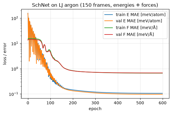
where \(E, \vec F_i\) are the reference energy and forces, \(\hat E\) the model energy, and the hyperparameter \(\rho\) balances the impact of two terms during optimization. The manuscript uses \(\rho = 0.01\), which the authors optimized empirically, to account for the different scales of the energy and forces. The magnitude of raw energies in the original SchNet training dataset are huge compared to those of their corresponding forces. After our per-atom standardization, the energy fluctuations (tens of meV) and force components (tens of meV/Å) have similar scales. So, we can set \(\rho = 1\) for our toy dataset.
Why do we train on forces after all? Each frame carries one energy label but \(3n\) force labels, and forces probe the local shape of the potential energy surface (as gradients of the energy). In the SchNet manuscript, adding forces at \(n{=}1000\) training frames improves energies more than going to \(n{=}50{,}000\) frames with energies alone. Our dataset, however, is tiny (< 1000 frames). So, we do simple full-batch gradient descent with Adam optimizer.
Let us implement the loss function and the training loop.
# Define a function to evaluate the mean absolute error (MAE) for energy and forces
def eval_mae(model, batch):
    '''(energy MAE per atom [meV/atom], force MAE [meV/Å]).'''

    # Unpack the batch into its components
    pos, species, edge_index, bvec, E_ref, F_ref = batch

    # Compute the energy and forces using the model
    E, F = energy_and_forces(model, pos, species, edge_index, bvec, len(E_ref))

    # Calculate the mean absolute error (MAE) for energy and forces
    e_mae = (E - E_ref).abs().mean().item() / n_atoms * 1e3
    f_mae = (F - F_ref).abs().mean().item() * 1e3
    return e_mae, f_mae

# Define a loss function that combines energy and force errors
def loss_fn(E, F, E_ref, F_ref, rho=1.0):
    '''Eq. (5): rho * ||E - E^||^2  +  (1/n) sum_i ||F_i - F^_i||^2   (mean over frames).'''

    # Compute the mean squared error (MSE) for energy and forces
    loss_E = ((E_ref - E) ** 2).mean()
    loss_F = ((F_ref - F) ** 2).sum(dim=-1).mean()         # (1/n) sum_i |F_i - F^_i|^2, mean over frames

    # Return the combined loss as a weighted sum of energy and force losses
    return rho * loss_E + loss_F
# Set up the optimizer, learning rate scheduler, and history tracking for
# training
optimizer = torch.optim.Adam(model.parameters(), lr=3e-3)
scheduler = torch.optim.lr_scheduler.CosineAnnealingLR(optimizer, T_max=600)
history = {"train E MAE [meV/atom]": [], "val E MAE [meV/atom]": [],
           "train F MAE [meV/Å]": [], "val F MAE [meV/Å]": []}

# Unpack the training batch into its components
pos, species, edge_index, bvec, E_ref, F_ref = train_batch

# Start the training loop for 600 epochs
t0 = time.time()
for epoch in range(1, 600 + 1):
    model.train(); optimizer.zero_grad()
    # Keep the compute graph: d(loss_F)/dpos
    E, F = energy_and_forces(model, pos, species, edge_index, bvec,
                             len(E_ref), create_graph=True)
    loss = loss_fn(E, F, E_ref, F_ref, rho=1.0)
    loss.backward()
    optimizer.step()
    scheduler.step()

    # Evaluation of training and validation MAE for energy and forces
    tr = eval_mae(model, train_batch)
    va = eval_mae(model, val_batch)
    for key, v in zip(history, (tr[0], va[0], tr[1], va[1])):
        history[key].append(v)
    if epoch % 100 == 0 or epoch == 599:
        print(f"epoch {epoch:4d}  loss {loss.item():.3e}   "
              f"val E MAE {va[0]:7.3f} meV/atom   val F MAE {va[1]:7.3f} meV/Å")

# Print the training time
print(f"training time: {time.time() - t0:.1f} s on {device}")
epoch  100  loss 3.464e-04   val E MAE   0.470 meV/atom   val F MAE   4.677 meV/Å
epoch  200  loss 6.694e-06   val E MAE   0.133 meV/atom   val F MAE   0.826 meV/Å
epoch  300  loss 4.336e-06   val E MAE   0.110 meV/atom   val F MAE   0.718 meV/Å
epoch  400  loss 3.772e-06   val E MAE   0.100 meV/atom   val F MAE   0.689 meV/Å
epoch  500  loss 3.596e-06   val E MAE   0.097 meV/atom   val F MAE   0.679 meV/Å
epoch  599  loss 3.569e-06   val E MAE   0.097 meV/atom   val F MAE   0.678 meV/Å
epoch  600  loss 3.569e-06   val E MAE   0.097 meV/atom   val F MAE   0.678 meV/Å
training time: 13.4 s on cuda
Let’s visualize the training and validation mean absolute errors (MAEs) for energy and forces.
# Use the convenient plotting function from course_utils
ax = plot_training_curves(history)

# Configure the plot with a title and adjust the layout
ax.set_title("SchNet on LJ argon (150 frames, energies + forces)")
ax.figure.tight_layout()
12.8.1. Force parity plot#
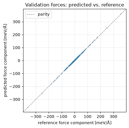
Let us now draw a parity plot which compares the predicted forces against the reference ones. In this plot, a perfect model should lie on the diagonal. We flatten all \(3n\) force components of every validation frame.
# Set the model to evaluation mode
model.eval()

# Get the predicted and reference forces in meV/Å
_, F_val = energy_and_forces(model, *val_batch[:4], len(val_batch[4]))
F_pred = F_val.detach().cpu().numpy().ravel() * 1e3
F_true = val_batch[5].cpu().numpy().ravel() * 1e3

# Visualize the predicted forces against the reference forces
fig, ax = plt.subplots(figsize=(4.6, 4.6))
lim = np.abs(F_true).max() * 1.1
ax.plot([-lim, lim], [-lim, lim], "--", color="gray", lw=1, label="parity")
ax.scatter(F_true, F_pred, s=8, alpha=0.4, color="C0", edgecolors="none")
ax.set_xlim(-lim, lim); ax.set_ylim(-lim, lim); ax.set_aspect("equal")
ax.set_xlabel("reference force component [meV/Å]")
ax.set_ylabel("predicted force component [meV/Å]")
ax.set_title("Validation forces: predicted vs. reference")
ax.legend()
ax.grid(True, alpha=0.3)
fig.tight_layout()

# Evaluate the final mean absolute error (MAE) for energy and forces on the
# validation set
e_mae, f_mae = eval_mae(model, val_batch)
print(f"final validation:  E MAE = {e_mae:.3f} meV/atom   |   F MAE = {f_mae:.3f} meV/Å")
final validation: E MAE = 0.097 meV/atom | F MAE = 0.678 meV/Å
12.9. Numerical verification of invariant energy and covariant forces#
We now used the course harness (course_utils.equivariance) to numerically test
the energy invariance and force covariance properties of SchNet in float64, in
order to separate genuine symmetry breaking from round-off errors:
Energy transforms as the trivial irrep
0e: \(\hat E(RX + \vec t\,) = \hat E(X)\) for random \(R \in O(3)\) (rotations and improper rotations/parity) and translations \(\vec t\).Forces transform as vectors
1o: \(\vec F(RX + \vec t\,) = R\, \vec F(X)\).
The wrapper functions rebuild the radius graph from the transformed positions, so the test covers the whole pipeline (graph construction included), not just the network forward pass.
Note: For \(l=1\) outputs, the harness compares against
o3.Irreps("1o").D_from_matrix(R). The e3nn’s matrix \(\to\) Euler angles \(\to\) Wigner-D conversion is itself only accurate to \(\approx 10^{-7}\): This (not the model) limits the tolerance of the harness check. Since for \(l = 1\), the Wigner D-matrix is the rotation matrix itself, we add a direct check \(\vec F(RX + \vec t\,) = R\,\vec F(X)\) against \(R\), which passes at fullfloat64precision.
# Create a deep copy of the trained model, convert it to double precision, move
# it to CPU, and set it to evaluation mode
model64 = copy.deepcopy(model).double().cpu().eval()

# Clone the positions from the first validation frame for testing
# float64 positions, (8, 3)
pos_test = val_frames[0]["pos"].clone()

# Create zero tensors for species and batch indices for the test positions
z_test = torch.zeros(n_atoms, dtype=torch.long)
b_test = torch.zeros(n_atoms, dtype=torch.long)

# pos -> E, shape (1,): irrep 0e
def energy_fn(pos):
    # Graph rebuilt after transform
    edge_index = radius_graph(pos, R_CUT)
    return model64(pos, z_test, edge_index, b_test, 1).reshape(1)

# pos -> F, shape (n, 3): irrep 1o
def force_fn(pos):
    edge_index = radius_graph(pos.detach(), R_CUT)
    _, F = energy_and_forces(model64, pos, z_test, edge_index, b_test, 1)
    return F

print("energy  E(RX + t) = E(X):")
assert_model_equivariant(energy_fn, pos_test, "0e", tol=1e-12)
print("forces  F(RX + t) = R F(X)  (harness; tol limited by e3nn's D_from_matrix ~1e-7):")
assert_model_equivariant(force_fn, pos_test, "1o", tol=1e-6)
energy  E(RX + t) = E(X):
equivariant!  (max error 8.327e-17 over random O(3) + translations elements)
forces  F(RX + t) = R F(X)  (harness; tol limited by e3nn's D_from_matrix ~1e-7):
equivariant!  (max error 7.296e-09 over random O(3) + translations elements)
7.296132954748291e-09
Now, let us directly check against the \(R\) itself (for \(l = 1\), the Wigner \(D\) is the rotation matrix):
# Get the reference forces for the test positions
F_ref = force_fn(pos_test)

# Run the test for 5 random rotations and translations, including improper rotations
err = 0.0
for _ in range(5):

    # Generate a random rotation matrix R
    R = o3.rand_matrix(dtype=torch.float64)

    # With a 50% chance, apply an improper rotation (parity test) by negating
    # the rotation matrix
    if torch.rand(()) < 0.5:
        R = -R

    # Generate a random translation vector t
    t = torch.randn(3, dtype=torch.float64)

    # Compute the maximum error between the transformed forces and the reference
    # forces
    err = max(err, (force_fn(pos_test @ R.T + t) - F_ref @ R.T).abs().max().item())

# Check that the maximum error is below the specified tolerance and print the
# result
assert err < 1e-12, err
print(f"Forces are exactly covariant: max |F(RX+t) - R F(X)| = {err:.3e}  (float64)")
Forces are exactly covariant: max |F(RX+t) - R F(X)| = 1.344e-16 (float64)
12.10. Summary#
In this lesson, we have learned:
Distances are E(3)-invariant (rotations, translations, and parity). So, any network built on \(\{Z_i, d_{ij}\}\) predicts invariant energies by construction.
SchNet architecture consists of atom-type embedding \(\to\) interaction blocks, each: atom-wise \(\to\) cfconv (\(\sum_j x_j \odot W(d_{ij})\), filters generated from a Gaussian-RBF distance expansion by a small ssp-MLP) \(\to\) atom-wise \(\to\) ssp \(\to\) atom-wise, with a residual connection \(\to\) atom-wise readout, sum-pooled to \(\hat E\).
Forces are generated by autograd as \(\vec F_i = -\partial\hat E/\partial\vec r_i\): They are conservative by construction, consistent with the energy, and automatically covariant (\(\vec F(RX) = R\vec F(X)\), which we have numerically verified the covariance property up to \(\approx 10^{-13}\)).
Training with the combined loss (weighted sum of energy and force losses) exploits the \(3n\) force labels per frame, where \(n\) is the number of atoms in the system. We standardized energies by a per-atom mean shift so the network doesn’t waste time learning a constant shift in the energies.
Next: In Lesson 07b, we discuss the environments, in which, the distance-only models do not perform well which motivates us to introduce DimeNet that incorporates angles into the model via directional message passing.
12.11. Exercises#
1. Energy-only training (Difficulty: 🌶️): Retrain with the force term removed (set its weight to zero, keep \(\rho = 1\)). How do the validation force errors compare? Relate your finding to Table 2 of the SchNet paper.
Solution
Set loss = rho * loss_E (or add a force_weight=0.0 factor). Energy MAE stays
reasonable, but force MAE degrades by a large factor: the model matches energies
of the 150 training geometries without matching the slope of the PES between
them. This mirrors the SchNet’s manuscript observation: a model trained on
energies alone using 1000 training datapoints has force errors an order of
magnitude worse than the energy+force model. This is why many modern interatomic
potentials train on forces as well.
2. Break the smoothness (Difficulty: 🌶️🌶️): Replace ssp by torch.relu in FilterNet and
the readout, and retrain the model. What happens to the force loss and the
parity plot? Why is this expected?
Solution
Training still runs (autograd differentiates ReLU almost everywhere, except at zero), but forces become piecewise-constant functions of the inputs with jumps. The training on the force loss requires second derivatives, which are zero almost everywhere for ReLU. Therefore, the gradients of the force term stop flowing through the filter shape and the force fit stalls/roughens. This is exactly why the authors of SchNet chose the \(C^\infty\) shifted softplus for nonlinearity.
3. Remove the cutoff function (Difficulty: 🌶️🌶️🌶️): Delete the f_cut factor in FilterNet and
retrain the model. Then, study the retrained model on a simple system that
crosses the cutoff: an isolated argon dimer. Fix atom A at the origin and
place atom B at \((d, 0, 0)\), sweeping \(d\) on a fine grid from 5.8 Å to 6.2
Å across \(r_\mathrm{cut} = 6\) Å (rebuild the radius graph with
radius_graph at each \(d\), as in the equivariance-check section). Plot the
model energy \(\hat E\) vs. \(d\). What do you see at \(d = 6\) Å, and why does it
matter for MD?
Solution
At \(d = r_\mathrm{cut}\) the dimer’s only edge vanishes from the radius graph. Without \(f_\mathrm{cut}\), the filter value is still non-zero there, so the energy curve jumps discontinuously at 6 Å (and beyond it, the two atoms are disconnected and \(\hat E\) is flat at twice the isolated-atom readout). The force (the derivative of the energy) is undefined/infinite at the jump point. In MD, this jump causes unphysical behavior and destroys energy conservation. With \(f_\mathrm{cut}\), the jump contribution vanishes smoothly (and the energy value and its derivative go to zero at \(r_\mathrm{cut}\)).