
18. Lesson 09a: Allegro as a Strictly Local Equivariant Potential#
What you will learn
Why message passing makes the receptive field grow as \(N_\text{layer} \times r_c\) and why that hurts parallel scaling for large systems.
Allegro’s strictly local decomposition of the energy into pairwise terms \(E_{ij}\), each computed by a deep equivariant network with no message passing between environments.
The two-track layer design: an invariant scalar latent-space track \(x^{ij}\) and an equivariant tensor latent-space track \(V^{ij}\), coupled once per layer by a weighted tensor product with spherical harmonics of the local environment.
Why scalar features may pass through arbitrary MLPs while \(\ell > 0\) features may not.
The scaling argument: independent pair terms allow embarrassingly parallel force evaluation and the Allegro paper’s 100-million-atom demonstration.
A side-by-side comparison of NequIP and Allegro.
Prerequisites:
Lesson 02a and 2b: irreps, spherical harmonics,
Lesson 04: equivariant nonlinearities, gates,
Lesson 05a: graphs, radial bases,
Lesson 08a: NequIP theory.
import sys; sys.path.insert(0, "..")

import matplotlib.pyplot as plt
import numpy as np
import torch
from e3nn import o3

from course_utils.equivariance import assert_equivariant, equivariance_error

torch.manual_seed(0)
# This is a theory notebook: the code is illustrative and cheap, so we use
# float64 everywhere — equivariance checks then sit at machine precision.
torch.set_default_dtype(torch.float64)
device = "cpu"
print(torch.__version__)
2.7.1+cu126
18.1. The cost of message passing: receptive fields#
Atom-centered message-passing neural networks (MPNNs), such as SchNet (Lesson 07a), DimeNet (Lesson 07b), NequIP (Lessons 08a-c) keep a hidden state \(\mathbf{h}_i^t\) on every central atom \(i\) and update it by exchanging messages along the edges of the atomic graph within a local cutoff radius. That is:
where \(\mathcal{N}(i)\) is the set of neighbors of atom \(i\) within the local cutoff radius, \(r_{c,l}\), \(\mathbf{e}_{ij}\) are edge features (typically functions of the interatomic distance \(r_{ij}\)), and \(M_t\), \(U_t\) are the learned message and update functions of layer \(t\).
After one layer (i.e., at iteration \(t=1\)), \(\mathbf{h}_i\) knows about atoms within \(r_{c,l}\); after two layers, it knows about atoms within \(2\,r_{c,l}\) (its neighbors’ neighborhoods), and so on. With \(N_\text{layer}\) message-passing layers, the effective cutoff radius is
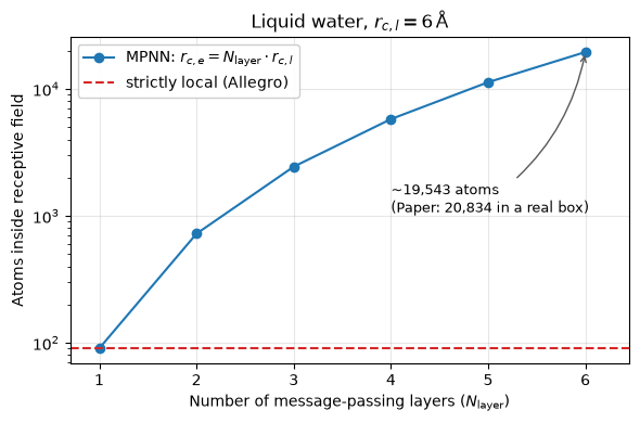
and the number of atoms inside the receptive field grows cubically in \(r_{c,e}\). For example, the liquid water at ambient conditions with a typical setting of \(N_\text{layer}=6\) and \(r_{c,l}=6\,\text{Å}\) gives \(r_{c,e} = 36\,\text{Å}\). Each atom then has \(\approx 96\) atoms in its local 6 Å environment but 20,834 atoms inside the extended 36 Å effective cutoff radius (receptive field) which affect the final state of the central atom and contribute to its local environment (impacting properties such as energy, forces, and other local physical quantities).
Let’s visualize the relationship between the number of atoms in the receptive field vs. the number of message-passing layers in a typical MPNN model for a liquid water system.
# Atoms / A^3  (~0.0334 molecules/A^3 x 3 atoms)
rho = 0.10

# Local cutoff in Angstroms
r_c = 6.0

# Number of message-passing layers
n_layers = np.arange(1, 7)

# Effective cutoff radius
r_eff = n_layers * r_c

# Number of atoms inside the receptive field
# ~ cubic growth
atoms_in_receptive_field = 4 / 3 * np.pi * r_eff**3 * rho

# Number of atoms in the strictly local environment (Allegro)
atoms_local = 4 / 3 * np.pi * r_c**3 * rho

# Visualization of the relationship between the number of atoms in the receptive
# field and the number of message-passing layers
fig, ax = plt.subplots(figsize=(6, 4))
ax.semilogy(n_layers, atoms_in_receptive_field, "o-", label=r"MPNN: $r_{c,e}=N_\mathrm{layer} \cdot r_{c,l}$")
ax.axhline(atoms_local, color="C3", ls="--", label="strictly local (Allegro)")
# Call out the deepest MPNN point from the empty wedge below the curve
ax.annotate(f"~{atoms_in_receptive_field[-1]:,.0f} atoms\n(Paper: 20,834 in a real box)",
            xy=(6, atoms_in_receptive_field[-1]), xytext=(4, 1340),
            fontsize=9, va="center",
            arrowprops=dict(arrowstyle="->", color="0.35",
                            connectionstyle="arc3,rad=0.2"))
ax.set_xlim(0.7, 6.45)
ax.set_xlabel(r"Number of message-passing layers ($N_\mathrm{layer}$)")
ax.set_ylabel(r"Atoms inside receptive field")
ax.set_title(r"Liquid water, $r_{c,l} = 6\,\mathrm{\AA}$")
ax.legend(loc="upper left", framealpha=0.95)
ax.grid(True, alpha=0.3)
fig.tight_layout()
18.1.1. Why this hurts parallel scaling#
Large-scale MD codes (e.g. LAMMPS) parallelize their work by spatial domain decomposition: each worker owns a region of space and communicates a “halo” of ghost atoms with its neighbors. The halo thickness must cover the interaction range of the potential:
For an MPNN, that range is \(r_{c,e} = N_\text{layer}\, r_{c,l}\). Every worker must access the high-dimensional hidden states \(\mathbf{h}_i\) of all \(\approx\) 20,000 atoms in the extended environment. It would also be worse for the force computations which are computed through back-propagation of the gradients along the same multi-hop graph which requires iterated communication at every step.
A strictly local model only needs the states associated with the \(\approx\) 96 atoms (in the example above, \(6^3 = 216\) pair states) inside a single cutoff sphere.
This is exactly why strictly local classical potentials and descriptor methods (e.g., Behler-Parrinello HDNNPs, GAP, SNAP, ACE, …) can scale to enormous systems.
18.2. Strictly local pairwise-energy decomposition#
The Allegro model decomposes the total potential energy of an into per-atom energy contributions,
where \(Z_i\) is the chemical species of atom \(i\), and \(\sigma_{Z_i}\) and \(\mu_{Z_i}\) denote per-species scale and shift parameters, respectively. Both \(\sigma_{Z_i}\) and \(\mu_{Z_i}\) may be trainable parameters.
Unlike most MLIPs, however, Allegro further decomposes each per-atom energy into pairwise energies, indexed by the central atom \(i\) and one of its neighbors \(j\):
Here, \(\sigma_{Z_i,Z_j}\) is the per-species-pair scale factor, which may also be a trainable parameter.
Atomic forces are the exact negative gradient of the total energy with respect to the atomic positions. As such, the Allegro’s force field becomes energy-conserving by construction:
From the theoretical construction, two points may become easy to misread:
While \(E_{ij}\) are indexed by atom \(i\) and \(j\), their value may depend on all neighboring atoms \(k \in \mathcal{N}(i)\) of the central atom \(i\). The network couples each pair to its full local environment, making Allegro a many-body potential.
\(E_{ij} \neq E_{ji}\), by design. \(E_{ij}\) depends on the environment of \(i\), while \(E_{ji}\) depends on the environment of \(j\). The two terms are computed independently and only their sum is physically meaningful.
So, in Allegro, the strict locality means that everything depends only on atoms within one cutoff sphere, no matter how deep the network architecture gets.
18.3. The coupled latent spaces#
Allegro processes each ordered pair \((i,j)\) with two coupled latent spaces:
track |
symbol |
content |
transformation |
|---|---|---|---|
scalar space |
\(x^{ij,L}\) |
invariant latent features of pair \((i,j)\) at layer \(L\) |
invariant (\(\ell = 0\)) |
tensor space |
\(V^{ij,L}_{n,\ell,p}\) |
equivariant features: \(n\) = channel, irrep \((\ell, p)\) with \(\ell = 0 \dots \ell_\text{max}\), parity \(p \in \{-1, 1\}\) |
Wigner matrices \(D^{(\ell)}(g)\), \(\times (\pm 1)\) for parity |
Why are there two latent spaces?
A scalar (\(\ell = 0\)) feature remains unchanged under rotations. Thus, any elementwise nonlinearity such as \(\tanh\), SiLU, a whole MLP etc. maps invariants to invariants. The scalar latent space side of the network can therefore use any ordinary deep neural network operation which are often cheap, expressive, and unconstrained.
An \(\ell > 0\) feature mixes its components under rotation. Applying a nonlinearity componentwise breaks equivariance, because \(\phi(D(g)\,V) \neq D(g)\,\phi(V)\) for a nonlinear \(\phi\). The tensor latent space side of the network is therefore restricted to the equivariant operations such as those we built in Lessons 03-04, which involved linear channel mixing within an irrep, and tensor products to combine irreps:
with the Wigner \(3j\) symbol as the coupling coefficients (equivalent to the Clebsch–Gordan coupling of Lesson 03a).
Each Allegro layer couples the scalar and tensor tracks in both directions: the scalar track generates the weights of the tensor-track tensor product, and the scalar (\(\ell=0\)) outputs of that tensor product are fed back into the scalar track.
Let’s first verify the asymmetry that motivates the design of the Allegro architecture.
# An elementwise nonlinearity is equivariant on scalars (0e) but NOT on vectors (1o)
err_scalars = equivariance_error(torch.tanh, "8x0e", "8x0e")
err_vectors = equivariance_error(torch.tanh, "8x1o", "8x1o")

# Print the equivariance errors for scalars and vectors
print(f"tanh on 8x0e: max equivariance error = {err_scalars:.2e}   (invariant --> fine)")
print(f"tanh on 8x1o: max equivariance error = {err_vectors:.2e}   (breaks equivariance!)")
tanh on 8x0e: max equivariance error = 0.00e+00   (invariant --> fine)
tanh on 8x1o: max equivariance error = 8.22e-01   (breaks equivariance!)
18.4. Initial two-body embedding#
Scalar space route (layer \(L=0\)): The atomic pair \((i,j)\) is embedded from its species pair \((Z_i, Z_j)\) and distance \(r_{ij}\),
where \(\Vert\) denotes concatenation, \(\mathrm{1Hot}(\cdot)\) is a one-hot encoding for species, \(B_n\) are Bessel radial basis functions, and \(u(r_{ij})\) is the smooth polynomial cutoff envelope (both from Lesson 05b; we implement them in 09b). Multiplying by \(u(r_{ij})\) makes the embedding and everything downstream go smoothly to zero at the cutoff.
Tensor space route (layer \(L=0\)): The initial equivariant features are a learned linear embedding of the spherical-harmonic projection of the central pair direction \(\hat{r}_{ij}\) (with \(\vec{r}_{ij} = \vec{r}_j - \vec{r}_i\), the convention used throughout this course):
Here, \(\vec{Y}^{\,ij}_{\ell,p}\) is the projection of \(\hat{r}_{ij}\) onto the real spherical harmonic of degree \(\ell\) (parity \(p = (-1)^\ell\); the \(m\) index is suppressed), \(n = 0, \dots, n_\text{equivariant}-1\) is the channel index, and the scalar weights, \(w\), are predicted from the scalar space route. This signifies the first instance of scalar \(\to\) tensor coupling in Allegro.
18.5. The Allegro layer#
Each Allegro tensor-product layer has four components:
an MLP that generates weights to embed the central atom’s environment,
an equivariant tensor product, which uses those weights,
an MLP that updates the scalar latent space with the scalar outputs of the tensor product,
an equivariant linear layer that mixes channels in the equivariant latent space.
Let’s go through each of these components in more details.
18.5.1. Tensor product with the embedded environment (Comps. 1 & 2)#
The tensor product in the tensor space route couples the pair features, \(V^{ij,L-1}\), to all other pairs \(ik\) in the environment of \(i\):
Because the tensor product is bilinear, the sum over neighbors can be pulled inside the parenthesized term. This is a special example of the density trick, which expresses the update as a single tensor product rather than one tensor product per neighbor:
The bracketed sum is the embedded environment of atom \(i\): a weighted spherical-harmonic projection of the atomic density around \(i\) similar to the projection used in ACE and SOAP frameworks. Note that the weights are not a fixed radial-chemical basis but are learned via the scalar space route:
where an embedded environment with a fixed and user-defined number of channels (\(n_\text{equivariant}\)) is constructed.
At layer \(L > 1\), \(x^{ik,L-1}\) already contains many-body information about the environment of \(i\). As such, the environment embedding becomes increasingly informative with increasing the network depth. All tensor-product paths satisfying \(|\ell_1 - \ell_2| \le \ell_\text{out} \le \ell_1 + \ell_2\), \(p_\text{out} = p_1 p_2\), and \(\ell_\text{out} \le \ell_\text{max}\) are candidates and which ones to include is a hyperparameter.
18.5.2. The latent MLP and tensor \(\to\) scalar coupling (Comp. 3)#
The scalar (\(\ell_\text{out}=0,\, p_\text{out}=1\)) outputs of the tensor product are concatenated with the previous equivariantlatent features and compressed back into the fixed-width scalar latent space route:
After each layer, the scalar latent route additionally uses a residual update, in which the new features are added to those of layer \(L-1\). Residual connections can help the scalar information propagate easily through depth.
18.5.3. Linear mixing (Comp. 4)#
The outputs of different tensor product paths, carrying the same irrep \((\ell, p)\), are mixed back to \(n_\text{equivariant}\) channels per irrep:
Here, \(\text{path}\) replaces \((\ell_1,p_1,\ell_2,p_2)\). Note what is absent here: no update ever reads features of pairs centered on other atoms and no information ever propagates beyond \(\mathcal{N}(i)\).
18.5.4. The Allegro layer in e3nn and irreps book-keeping#
Let’s instantiate the equivariant core of one Allegro-style layer and watch the
irreps flow through it. We use \(\ell_\text{max}=2\), \(C = 4\) channels. The
channel index, \(n\), is shared between the two tensor product inputs (e3nn’s
"uuu" connection mode: channel \(n\) of \(V\) couples only to channel \(n\) of the
environment). We keep only paths whose output irrep is one of the irreps of
\(\vec{Y}\) (\(0e\), \(1o\), \(2e\)) which will be our hyperparameter choice.
First, we create our channel-wise tensor product function.
def channelwise_tp(irreps_V, irreps_env, allowed):
    """Weight-free channel-wise tensor product with all allowed paths."""

    # Convert the allowed irreps to a set for faster lookup
    allowed = {o3.Irrep(ir) for ir in allowed}

    # Initialize the output irreps and instructions for the tensor product
    irreps_out, instructions = [], []
    for i1, (mul, ir1) in enumerate(irreps_V):
        for i2, (_, ir2) in enumerate(irreps_env):

            # Selection rules (Lesson 03)
            for ir_out in ir1 * ir2:

                # Check if this output irrep is in the allowed set
                if ir_out in allowed:

                    # Add an instruction for this allowed path
                    instructions.append((i1, i2, len(irreps_out), "uuu", False))

                    # Record the output irrep for this path
                    irreps_out.append((mul, ir_out))

    # Return the tensor product object with the computed output irreps and
    # instructions
    return o3.TensorProduct(irreps_V, irreps_env, o3.Irreps(irreps_out), instructions,
                            internal_weights=False, shared_weights=False)
We now use the channel-wise tensor product and the linear mixing layer to build the equivariant core of the Allegro-style layer.
# n_equivariant channels
C = 4

# 1x0e + 1x1o + 1x2e
irreps_Y = o3.Irreps.spherical_harmonics(2)

# Tensor latent route
irreps_V = o3.Irreps([(C, ir) for _, ir in irreps_Y])

# Embedded environment: C weighted copies of Y
irreps_env = irreps_V

# Channel-wise tensor product with all allowed paths
tp = channelwise_tp(irreps_V, irreps_env, [ir for _, ir in irreps_V])

# Every path visible, zero weights inside
print(tp)

# Count the number of scalar (0e) paths in the tensor product
n_scalar_paths = sum(mul for mul, ir in tp.irreps_out if ir == o3.Irrep("0e"))

# Print the number of scalar (0e) paths and the total number of channel-wise paths
print(f"\nirrep-level paths: {len(tp.instructions)} (e3nn counts {len(tp.instructions)} x C = "
      f"{C * len(tp.instructions)} channel-wise paths above)")
print(f"scalar (0e) outputs fed back to the scalar track: {n_scalar_paths}")

# Linear mixing of the tensor product output back to the tensor latent route
linear_mix = o3.Linear(tp.irreps_out, irreps_V)

# Print the linear mixing layer
print(linear_mix)
TensorProduct(4x0e+4x1o+4x2e x 4x0e+4x1o+4x2e -> 4x0e+4x1o+4x2e+4x1o+4x0e+4x2e+4x1o+4x2e+4x1o+4x0e+4x2e | 44 paths | 0 weights)

irrep-level paths: 11 (e3nn counts 11 x C = 44 channel-wise paths above)
scalar (0e) outputs fed back to the scalar track: 12
Linear(4x0e+4x1o+4x2e+4x1o+4x0e+4x2e+4x1o+4x2e+4x1o+4x0e+4x2e -> 4x0e+4x1o+4x2e | 176 weights)
Having the building blocks of Allegro-style layers, we can test them by applying them to a sample input and observing the flow of irreps through the layer.
# Trace one layer update for a central atom i with 5 neighbors (fake data, real
# shapes)
n_edges, latent_dim = 5, 16

# Scalar latents of the pairs (i,k)
x_ik = torch.randn(n_edges, latent_dim)

# Displacement vectors
r_ik = torch.randn(n_edges, 3)

# Spherical harmonics of the displacement vectors
Y_ik = o3.spherical_harmonics(irreps_Y, r_ik, normalize=True, normalization="component")

# Weights from the scalar latent route
w = torch.nn.Linear(latent_dim, C * len(irreps_Y))(x_ik)
w = w.reshape(n_edges, C, len(irreps_Y))

# Embedded environment
blocks, idx = [], 0
for m, (_, ir) in enumerate(irreps_Y):

    #  Weight each Y irrep per channel...
    blk = w[:, :, m:m+1] * Y_ik[:, None, idx:idx + ir.dim]
    blocks.append(blk.reshape(n_edges, C * ir.dim))
    idx += ir.dim

#   ...then sum over neighbors k
env_i = torch.cat(blocks, dim=-1).sum(0, keepdim=True)

# Current pair features V^{ij,L-1}
V_ij = irreps_V.randn(1, -1)

# V x (embedded environment)
tp_out = tp(V_ij, env_i)

# 0e slice -> latent MLP input
scalars = tp_out[:, :n_scalar_paths]

# Linear mixing of the tensor product output to get the new pair features V_new
V_new = linear_mix(tp_out)

# Print shapes and irreps of the intermediate features
for name, t, irr in [("x_ik (scalar track)", x_ik, "-"), ("Y_ik", Y_ik, irreps_Y),
                     ("env_i", env_i, irreps_env), ("V_ij", V_ij, irreps_V),
                     ("tp_out", tp_out, tp.irreps_out.simplify()),
                     ("-> scalars to x-track", scalars, f"{n_scalar_paths}x0e"),
                     ("-> V_new (mixed)", V_new, irreps_V)]:
    print(f"{name:24s} shape {tuple(t.shape)!s:12s} irreps {irr}")
x_ik (scalar track)      shape (5, 16)      irreps -
Y_ik                     shape (5, 9)       irreps 1x0e+1x1o+1x2e
env_i                    shape (1, 36)      irreps 4x0e+4x1o+4x2e
V_ij                     shape (1, 36)      irreps 4x0e+4x1o+4x2e
tp_out                   shape (1, 140)     irreps 4x0e+4x1o+4x2e+4x1o+4x0e+4x2e+4x1o+4x2e+4x1o+4x0e+4x2e
-> scalars to x-track    shape (1, 12)      irreps 12x0e
-> V_new (mixed)         shape (1, 36)      irreps 4x0e+4x1o+4x2e
18.5.5. Equivariance check#
An equivariant Allegro layer must be built from equivariant building blocks (tensor product and linear mixing). We test the O(3)-equivariance of these two units with the course harness, treating the pair features and the environment as one concatenated input.
# Concatenated (V, env) input
irreps_in = irreps_V + irreps_env

# Split the concatenated input into V and env parts
split = lambda z: (z[:, :irreps_V.dim], z[:, irreps_V.dim:])

# Equivariance check for the tensor product and linear mixing units
print("tensor product:                     ", end="")
assert_equivariant(lambda z: tp(*split(z)), irreps_in, tp.irreps_out)
print("tensor product + mixing:            ", end="")
_ = assert_equivariant(lambda z: linear_mix(tp(*split(z))), irreps_in, irreps_V)
tensor product:                     equivariant!  (max error 2.576e-14 over random O(3) elements)
tensor product + mixing:            equivariant!  (max error 1.377e-14 over random O(3) elements)
18.6. Readout and forces#
After \(N_\text{layer}\) layers, only the output of the scalar latent route is read out:
The pairwise energies are aggregated into \(E_\text{system}\), and forces come from automatic differentiation,
Because every quantity that depends on the atomic pairs is multiplied by the envelope \(u(r)\), they fade in and out smoothly as atoms cross the cutoff. This is a hard requirement for stable molecular dynamics simulations (Lesson 05b).
It is important to note that the tensor latent route has no direct path to the energy: its job is to inject symmetry-resolved geometric information into the scalars, layer after layer.
18.7. How strict locality enables efficient parallelization?#
Since \(E_\text{system} = \sum_{i,j} E_{ij}\) (ignoring the scale/shift coefficients for clarity), the force on any atom \(a\) becomes:
and \(\nabla_a E_{ij} \neq 0\) only if \(a\) is inside the single cutoff sphere of the central atom \(i\). Pair-wise terms with different centers are completely independent. Therefore, they can be computed by different workers with only standard short-range halo exchange that involves no multi-hop propagation of hidden states or gradients.
The Allegro manuscript summarizes the cost of a given Allegro model as:
\(\mathcal{O}(N)\) in the number of atoms \(N\) (versus \(\mathcal{O}(N^2)\) for global-descriptor methods like sGDML),
\(\mathcal{O}(M)\) in the number of neighbors \(M\) per atom (versus \(\mathcal{O}(M^2)\) for models with explicit angular terms such as DimeNet, or attention over pairs),
\(\mathcal{O}(1)\) in the number of chemical species \(S\) (versus \(\mathcal{O}(S^2)\) for SOAP, and \(\mathcal{O}(S^{\text{bodyorder}-1})\) for ACE). Here, chemical species enter only through the learned two-body embedding at the cost of pair (rather than atom) featurization. As such, there is a larger memory footprint per atom in Allegro.
Table 4 and Fig. 5 of the Allegro manuscript show the timins on the MD simulation of \(\text{Li}_3\text{PO}_4\) with 421,824 atoms across 1-64 GPUs with strong scaling, a 50-million-atom \(\text{Li}_3\text{PO}_4\) box, and Ag with 100,640,512 atoms on 128 GPUs. The same (small, 1-layer) \(\text{Li}_3\text{PO}_4\) model reproduces AIMD structure (RDF/ADF) and Li-ion kinetics (MSD). Accuracy does not appear to be sacrificed either: on revMD-17 Allegro matches or beats NequIP on force MAE for most molecules (Table 1), and on QM9 even a single-layer Allegro outperforms deep MPNNs and transformers (Table 3).
18.8. A Quick Comparison of NequIP and Allegro#
The following table provides a quick comparison of the key features and trade-offs between NequIP and Allegro.
topic |
NequIP (equivariant MPNN, Lesson 08) |
Allegro (strictly local) |
|---|---|---|
features live on |
atoms: \(\mathbf{h}_i\) |
ordered pairs: \(x^{ij}\), \(V^{ij}_{n,\ell,p}\) |
information exchange |
messages hop atom \(\to\) atom, once per layer |
none between environments and layers revisit the same \(\mathcal{N}(i)\) |
receptive field |
\(N_\text{layer} \times r_{c,l}\) (grows with depth) |
\(r_{c,l}\) (independent of depth) |
many-body order |
grows implicitly with hops |
grows explicitly with layers: \(N_\text{layer}\) iterated tensor products \(\leftrightarrow\) ACE-like products \(\vec{Y}^{ij} \otimes \vec{Y}^{ik_1} \otimes \cdots\) |
MD communication |
multi-hop state + gradient exchange across workers |
independent pair-wise terms with standard short-range halo |
parallel scaling |
limited by receptive field |
\(\mathcal{O}(N)\), demonstrated to \(10^8\) atoms using 128 GPUs |
accuracy (Allegro manuscript) |
best on some revMD-17 energies |
matches/beats NequIP forces on revMD-17; beats MPNNs on QM9 benchmark set |
It is important to keep in mind what Allegro gives up in becoming a strictly local model. A message-passing network can, in principle, carry information beyond the local cutoff \(r_{c,l}\) (up to \(r_{c,e}\)) which allows capturing genuinely long-range effects (electrostatics, charge transfer, etc.) within the receptive field. In Allegro, anything beyond the local cutoff sphere is invisible to the model entirely: it is an important physical design choice not a mere hyperparameter selection.
18.9. Summary#
In this lesson, we have learned:
the MPNN’s receptive fields grow as \(N_\text{layer} \times r_{c,l}\). It offers decent accuracy which comes with a hefty communication cost. It is often challenging to parallelize MPNNs and scale them to large systems.
Allegro decomposes energy into pairwise terms \(E_{ij}\), computed strictly from one local environment: The model captures many-body effects while remaining strictly local.
Each Allegro layer runs with two coupled latent space tracks: scalars \(x^{ij}\), involviong conventional deep neural network operations such as free-form MLPs, and tensors \(V^{ij}\), comprised of tensor products and linear mixing only.
There is a bidirectional coupling cycle between scalar and tensor features: the scalar latent space track generates the environment-embedding weights, used in the equivariant tensor products, and the scalar \(0e\) part of tensor product outputs is fed back to the latent MLP to update the scalar features.
The central operation in Allegro is one channel-wise tensor product per pair-wise feature, i.e., \(V^{ij} \otimes \big(\sum_k w^{ik} \vec{Y}^{ik}\big)\), which we implemented and verified its correctness in e3nn.
Strict locality makes pair-wise terms independent which enables linear scaling and massive parallelism (up to 100M atoms), at state-of-the-art accuracy.
Next: In Lesson 09b, we implement a simplified but complete version of Allegro model in e3nn, verify its symmetries and cutoff smoothness, and train it on energies and forces, simultaneously using the LJ argon dataset and the same protocol adopted in Lesson 08b.
18.10. Exercises#
1. Receptive fields (Difficulty: 🌶️): A NequIP model uses 5 layers with \(r_{c,l} = 5\,\text{Å}\) on liquid water (\(\rho \approx 0.1\) atoms/Å\(^3\)). How many atoms are in the receptive field of one atom? How many are visible to an Allegro model with the same cutoff and any number of layers?
Solution
\(r_{c,e} = 25\) Å and \(N/V=\rho \Rightarrow N = \frac{4}{3}\pi (25)^3 \times 0.1 \approx 6{,}500\) atoms for NequIP. Allegro sees \(\frac{4}{3}\pi (5)^3 \times 0.1 \approx 52\) atoms regardless of the network depth (number of layers). Increasing the depth in Allegro increases the body-order of the interactions within those \(\approx\) 52 atoms, not their range.
2. Selection rules in the Allegro layer (Difficulty: 🌶️): For \(\ell_\text{max} = 2\) with spherical harmonics parities (\(0e, 1o, 2e\)), list all output irreps of \(1o \otimes 1o\) and \(2e \otimes 1o\). Our simplified layer drops any output irrep not in \(\{0e, 1o, 2e\}\). Which products get (partially) discarded, and why is discarding paths still exactly equivariant?
Solution
\(1o \otimes 1o = 0e + 1e + 2e\). The pseudovector \(1e\) is discarded. \(2e \otimes
1o = 1o + 2o + 3o\). Both \(2o\) (\(\ell \le \ell_\text{max}\) but odd-parity
\(\ell=2\)) and \(3o\) (\(\ell > \ell_\text{max}\)) are discarded. Each tensor product
path, \((\ell_1,p_1) \otimes (\ell_2,p_2) \to (\ell_\text{out},p_\text{out})\), is
individually equivariant and is built from a complete block of Clebsch-Gordan/3j
coefficients. Thus, keeping any subset of paths keeps the map equivariant. Which
paths to keep, nonetheless, is a hyperparameter choice. You can verify it with
channelwise_tp and assert_equivariant we defined earlier.
3. Asymmetric pair energies (Difficulty: 🌶️): List the set of atoms that influence \(E_{ij}\) and the set that influences \(E_{ji}\). Using \(\vec{F}_a = -\sum_{i,j} \nabla_a E_{ij}\), which pair-wise terms can a worker that owns atom \(a\)’s atomic neighborhood environment region compute without communication, and what must be exchanged with neighboring workers?
Solution
\(E_{ij}\) depends on \(\{i\} \cup \mathcal{N}(i)\) (all atoms within the cutoff radius \(r_{c,l}\) of the central atom \(i\), including \(j\)). Similarly, \(E_{ji}\) dependes on \(\{j\} \cup \mathcal{N}(j)\). These sets are different, and most often, \(E_{ij} \neq E_{ji}\). A processing worker can compute all pair-wise terms whose center \(i\) lies within its domain, provided that it also holds the ghost copies of atoms within \(r_{c,l}\) of its boundary (one halo). The gradients \(\nabla_a E_{ij} \neq 0\) only when \(a \in \{i\} \cup \mathcal{N}(i)\). Therefore, the atomic force contributions to ghost atoms are sent back to the worker that owns the corresponding atom \(a\) with a single reduction with no iterated communication.
18.11. References#
Batatia et al., The design space of E(3)-equivariant atom-centred potentials (2022)