
20. Lesson 10a: The Atomic Cluster Expansion (ACE)#
What you will learn
How the energy of a set of atoms is organized as a body-order expansion, and why an explicit summation over \(K\)-body terms costs \(\mathcal{O}(N_c^{K})\).
The construct of a one-particle basis defined as a radial basis times spherical harmonics: \(\phi_{nlm}(\vec r) = R_{nl}(r)\,Y^{(l)}_m(\hat r)\).
The density trick: Projecting the neighbor density onto the one-particle basis yields the atomic base, \(A_{i,nlm}\). The product of atomic bases gives the \((\nu+1)\)-body descriptors at a linear cost with respect to the number of neighbors.
Symmetrization: Contracting the atomic bases with (generalized) Clebsch–Gordan couplings yields the rotation- and inversion-invariant \(B\)-basis.
Why the \(B\)-basis is complete and how linear ACE models are built on it.
How ACE relates to message passing, which is the bridge to MACE in Lesson 10b.
Prerequisites:
Lesson 02b: Spherical harmonics,
Lessons 03a and 03b: Tensor products and Clebsch–Gordan coefficients,
Lesson 05b: Radial bases and cutoffs,
Lessons 08a and 09a: NequIP and Allegro, for the comparison in the final section.
import sys; sys.path.insert(0, "..")

import math
import matplotlib.pyplot as plt
import torch
from e3nn import o3

from course_utils.equivariance import assert_model_equivariant, model_equivariance_error
from course_utils.plotting import scene3d, draw_point_cloud, show3d

torch.manual_seed(0)
# This is a theory notebook and the code base is tiny. So, we use float64
# everywhere and the equivariance checks stay within machine precision.
torch.set_default_dtype(torch.float64)
device = "cpu"
print(f"torch {torch.__version__}")
torch 2.7.1+cu126
20.1. The body-order expansion of the energy#
The atomic cluster expansion theory (ACE) is based on its classical many-atom counterpart. Here, the total energy of a system of \(N\) atoms is expressed as
where \(\vec r_i\) is the position of atom \(i\), \(V_0\) is a constant, \(V^{(1)}\) is a chemical potential, and the potentials \(V^{(2)}, V^{(3)}, \dots\) are symmetric functions that vanish when two indices coincide. A term \(V^{(K)}\), involving \(K\) atoms, is called a \(K\)-body term. Regrouping the equation above around each atom gives the site energy,
with \(E = \sum_i E_i\) after absorbing \(V_0\). Once a cutoff radius, \(r_c\), is introduced, the sums run over the \(N_c\) neighbors of atom \(i\). Two factors make this expansion difficult to use in practice:
Slow convergence: For bulk metals, terms up to \(K > 15\) may be required.
Exponential cost: The order-\((K+1)\) term is a \(K\)-fold sum over neighbors and costs \(\mathcal{O}(N_c^{K})\). With \(N_c \approx 10^2\) to \(10^3\) in close-packed materials, anything beyond \(K = 3\) is prohibitive.
The ACE theory removes the second obstacle and helps with the first one by making high order terms more affordable.
20.1.1. The environment of atom \(i\)#
The site energy is a function of the environment \(\sigma = (\vec r_{i1}, \vec r_{i2}, \dots)\), and the set of displacement vectors \(\vec r_{ij} = \vec r_j - \vec r_i\) from atom \(i\) to its neighbors. \(E_i(\sigma)\) must be invariant under permutations of like neighbors and under the rotations and reflections of \(O(3)\). ACE builds in both types of invariances by construction.
20.2. The one-particle basis \(\phi_{nlm}\)#
ACE expands \(E_i(\sigma)\) in products of a complete basis of single-bond functions \(\phi_v(\vec r)\). A cluster basis function for a cluster of \(K\) bonds is can be expressed as
where \(\alpha = (j_1,\dots,j_K)\) lists the neighbors and \(\boldsymbol\nu = (v_1,\dots,v_K)\) the basis indices. For the single-bond basis, the following separable product of radial and angular functions can be adopted [Drautz, Phys. Rev. B 99, 014104 (2019)],
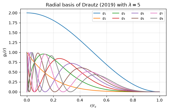
where, \(R_{nl}\) denotes the radial functions and \(Y^{(l)}_m\) stands for the spherical harmonics, \(r = |\vec r|\), and \(\hat r = \vec r / r\). These are exactly the objects we introduced in Lessons 02b and 05b. The radial functions are often built from a polynomial basis functions with a cosine cutoff,
where \(T_k\) are Chebyshev polynomials of the first kind and
are the rescaling functions (shown as \(x\) for brevity), with sharpness \(\lambda\) sample small distances more densely. As such, \(R_{nl}\) becomes a linear combination \(R_{nl} = \sum_k c_{nlk}\, g_k\). In this lesson, we take \(R_{nl} = g_n\), to make it simpler and independent of \(l\). Note that in Drautz, Phys. Rev. B 99, 014104 (2019), complex spherical harmonics are used while e3nn uses the real ones. We quote the equations as written there and explicitly state where the \((-1)^m\) structure matters and how they simplify in the real basis.
Let’s implement the radial basis functions in PyTorch
def drautz_radial_basis(r, n_max, r_c, lam=5.0):
    """g_1, ..., g_n_max of Drautz ."""

    # Rescaling function
    x = 1 - 2 * ((torch.exp(-lam * (r / r_c - 1)) - 1) / (math.exp(lam) - 1))

    # Cosine cutoff
    envelope = (1 + torch.cos(math.pi * r / r_c)) * (r < r_c)

    # g_1
    g = [envelope]

    # T_0, T_1
    T_prev, T_curr = torch.ones_like(x), x

    # Loop over k = 2, ..., n_max
    for k in range(2, n_max + 1):

        # g_k uses T_{k-1}
        g.append(0.25 * (1 - T_curr) * envelope)

        # Chebyshev recursion
        T_prev, T_curr = T_curr, 2 * x * T_curr - T_prev

    # Returns shape (*r.shape, n_max)
    return torch.stack(g, dim=-1)
The implementation allows us to also visualize the radial basis functions
# Set the cutoff radius
r_c = 5.0

# Create a grid of distances up to the cutoff radius
r_grid = torch.linspace(0.0, r_c, 400)

# Compute the radial basis functions for n_max=8
g_plot = drautz_radial_basis(r_grid, n_max=8, r_c=r_c)

# Plot the radial basis functions
fig, ax = plt.subplots(figsize=(6, 4))
for k in range(8):
    ax.plot(r_grid / r_c, g_plot[:, k], label=rf"$g_{{{k + 1}}}$")
ax.set_xlabel(r"$r / r_c$")
ax.set_ylabel(r"$g_k(r)$")
ax.set_title(r"Radial basis of Drautz (2019) with $\lambda = 5$")
ax.legend(ncols=4, fontsize=8)
ax.grid(alpha=0.3)
fig.tight_layout()
20.3. The density trick: from \(\mathcal{O}(N_c^{\nu})\) to \(\mathcal{O}(N_c)\)#
Arguably, the denisty trick is the key insight from the ACE framework. Expanding \(E_i\) in the cluster basis with unrestricted neighbor sums gives,
Evaluated naively, the order-\(\nu\) term is a \(\nu\)-fold sum over neighbors with \(N_c^{\nu}\) terms. Defining the atomic basis, \(A_{iv}\), as the projection of the basis functions onto the neighbor density, \(\rho_i\), we can write
where
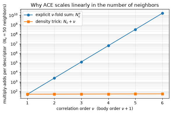
The atomic basis functions are expressed as a single sum over neighbors, a 2-body quantity (center plus one neighbor) which are computed once in \(\mathcal{O}(N_c)\) per basis function. The trick is that the unrestricted \(\nu\)-fold sums in the site energy expansion above can be reordered, using
to factorize the site energy expansion into a polynomial in \(A_{iv}\), with each set of terms carrying its own summation index as
Since the expansion coefficients, \(c^{(\nu)}_{v_1 \dots v_\nu}\), are symmetric with respect to the indices \(v_1, \dots, v_\nu\), an ordered sum \(v_1 \ge v_2 \ge \dots\) already covers every distinct combination of basis functions. The direction of the ordering is purely conventional: the coefficients and the product \(A_{iv_1} A_{iv_2} \cdots\) are both symmetric. So, both \(v_1 \ge v_2 \ge \dots\) and \(v_1 \le v_2 \le \dots\) enumerate the same terms. We follow Drautz’s descending ordering convention for consistency.
Building all atomic basis functions, \(A_{iv}\), costs \(\mathcal{O}(N_c \, n_{\text{1p}})\) for \(n_{\text{1p}}\) one-particle basis functions, and each product of \(\nu\) basis functions costs \(\mathcal{O}(\nu)\), independent of \(N_c\). Therefore, a \((\nu+1)\)-body descriptor will cost the same as that of a pair descriptor. This is why ACE scales linearly with the number of neighbors, irrespective of the order of the expansion.
The scaling advantage and potential speed-up in ACE’s density trick comes at a cost. Note that the neighbor sums in the first site energy expression above are unrestricted: every index \(j_\xi\) runs over all neighbor indices. Thus, the same neighbor can appear more than once in a product. For the second-order term, splitting off the terms with \(j_1 = j_2\) gives
The first sum couples the central atom \(i\) to two different neighbors, which is the 3-body term of the true many-body expansion. The second sum is the diagonal term, in which a neighbor effectively interacts with itself. Each tem in this summation depends on a single bond vector, \(\vec r_{ij}\). Therefore, it only amounts to a 2-body quantity with no counterpart in the original ACE expression. These self-interaction terms are the price of adopting the density trick. Fortunately, these terms are harmless in practice. A product of two one-particle functions of the same bond, is itself a function of that one bond. AS such, it can be expanded in the one-particle basis,
where the expansion coefficients, \(a^{v}_{v_1 v_2}\), are fixed numbers. The expansion is exact for a complete basis and approximate if truncated. Summing over the neighbor indices turns the diagonal term into \(\sum_v a^{v}_{v_1 v_2}\, A_{iv}\), which has exactly the form of a first-order term. When the model is fit, its contribution is simply absorbed into the first-order coefficients \(c^{(1)}_v\). The same argument holds at every order: a \(\nu\)-fold product with repeated neighbors collapses onto terms of lower order. As a result, self-interaction terms can change the expansion coefficients, \(c^{(\nu)}\), but cannot change the functions the expansion can represent.
Let’s build a toy atomic environment consisting of a central atom and its neighbors and verify the aforementioned properties of the basis functions, numerically
# A toy atomic environment: one central atom (origin) + N_neigh neighbors inside r_c.
N_neigh, r_c, n_max, l_max = 10, 5.0, 4, 3

# Create random neighbor positions in 3D space
directions = torch.randn(N_neigh, 3)

# Normalize the directions to unit vectors
directions = directions / directions.norm(dim=-1, keepdim=True)

# Generate random radii for the neighbors within the cutoff radius
# radii in [1.5, 4.5] < r_c
radii = 1.5 + 3.0 * torch.rand(N_neigh, 1)

# Compute the displacement vectors from the central atom to each neighbor
# Displacement vectors r_ij = r_j - r_i
vecs = radii * directions

# Visualize the toy atomic environment in 3D
fig = scene3d()
draw_point_cloud(vecs, fig=fig, color="C0", label="neighbors j")
draw_point_cloud(torch.zeros(1, 3), fig=fig, color="C3", size=12,
                 label="central atom i")
show3d(fig, title=f"Toy environment: {N_neigh} neighbors of atom i")
print("neighbor distances:", radii.squeeze().sort().values.numpy().round(2))
neighbor distances: [1.62 2.07 2.27 2.59 3.79 3.84 4.09 4.14 4.46 4.49]
20.3.1. The atomic base \(A_{i,nlm}\) in e3nn#
With \(v = (nlm)\) and \(R_{nl} = g_n\), the atomic basis can be expressed as
where we drop the constant \(\sqrt{4\pi}\) since it can be absorbed into the coefficients. In e3nn, this translates into a radial basis times spherical harmonics, summed over neighbors. Since \(Y^{(l)}\) has parity \((-1)^l\), the \(A\)’s for fixed \(n\) carry the irreps \(0e + 1o + 2e + 3o\), making the atomic basis equivariant.
# Create a list of angular momenta l = 0, 1, ..., l_max
ls = list(range(l_max + 1))

# Create the irreps for the spherical harmonics Y_lm and the atomic base A_{nlm}
# Y_lm is a spherical harmonic of degree l and order m
# A_{nlm} is the atomic base function for a given n, l, and m

# Parity of Y^(l) is (-1)^l
irreps_Y = o3.Irreps("1x0e+1x1o+1x2e+1x3o")

# n-major layout
irreps_A = o3.Irreps("+".join([str(irreps_Y)] * n_max))

def atomic_base(vecs):
    """A_{nlm} = sum_j g_n(r_j) Y_lm(r_j^)"""
    # Compute the radial basis functions g_n(r_j)
    r = vecs.norm(dim=-1)                                            # (N,)
    g = drautz_radial_basis(r, n_max=n_max, r_c=r_c)                 # (N, n_max)

    # Compute the spherical harmonics Y_lm(r_j^)
    Y = o3.spherical_harmonics(ls, vecs, normalize=True,
                               normalization="component")            # (N, 16)

    # Sum over neighbors j
    A = torch.einsum("jn,jy->ny", g, Y)

    # Returns a flat vector of irreps ``irreps_A`` (n-major: [n=1: 0e+1o+2e+3o,
    # n=2: ..., ...])
    return A.reshape(-1)


# Compute the atomic base A_{nlm} for the toy environment
A = atomic_base(vecs).reshape(n_max, irreps_Y.dim)

# Print the shape of the atomic base and the number of irreps per n
print(f"A-basis: {tuple(A.shape)}  =  (n_max, (l_max+1)^2);  irreps per n: {irreps_Y}")
print("Cost: one pass over", N_neigh, "neighbors --> O(N_c), a 2-body quantity")
A-basis: (4, 16)  =  (n_max, (l_max+1)^2);  irreps per n: 1x0e+1x1o+1x2e+1x3o
Cost: one pass over 10 neighbors --> O(N_c), a 2-body quantity
Any new equivariant object in this course gets an immediate numerical check,
\(A(g\,\sigma) = D(g)\,A(\sigma)\) for random elements, \(g \in O(3)\). Inversions
are included. Thus, the odd-\(l\) channels must flip sign. Translations are not
checked here because the atomic_base() takes displacement vectors, \(\vec
r_{ij}\), which makes them translation invariant by construction.
assert_model_equivariant(atomic_base, vecs, irreps_A, tol=1e-10, translation=False)
equivariant! (max error 2.842e-14 over random O(3) elements)
2.842170943040401e-14
20.3.2. Verifying the density trick factorization numerically#
We now check the density trick exactly: explicit double and triple sums over neighbor pairs and triples must equal products of \(A\)’s. We also evaluate the restricted sum with \(j_1 \ne j_2\), the true pair term, which differs from \(A_{v_1} A_{v_2}\) by exactly the self-interaction diagonal \(\sum_j \phi_{v_1}(\vec r_{ij})\phi_{v_2}(\vec r_{ij})\).
# One-particle basis values phi_{v}(r_ij) for every neighbor
# Shape (N_neigh, # n_v)
r = vecs.norm(dim=-1)

# Compute the one-particle basis values phi_{v}(r_ij) for every neighbor
phi = (drautz_radial_basis(r, n_max, r_c).unsqueeze(-1)
       * o3.spherical_harmonics(ls, vecs, True, normalization="component").unsqueeze(1))

# v = (n, lm) flattened, n_v = 64
phi = phi.reshape(N_neigh, -1)

# A_v = sum_j phi_v
A_flat = phi.sum(dim=0)

# Three arbitrary basis indices (n, lm) flat
v1, v2, v3 = 1, 20, 42

# Compute the explicit double and triple sums over neighbor pairs and triples
explicit_2 = sum(phi[j1, v1] * phi[j2, v2] for j1 in range(N_neigh) for j2 in range(N_neigh))
explicit_3 = sum(phi[j1, v1] * phi[j2, v2] * phi[j3, v3]
                 for j1 in range(N_neigh) for j2 in range(N_neigh) for j3 in range(N_neigh))

print(f"nu=2:  explicit double sum ({N_neigh ** 2} terms)  = {explicit_2: .10e}")
print(f"       A_v1 * A_v2         (2 factors)  = {A_flat[v1] * A_flat[v2]: .10e}\n")
print(f"nu=3:  explicit triple sum ({N_neigh ** 3} terms) = {explicit_3: .10e}")
print(f"       A_v1 * A_v2 * A_v3  (3 factors)  = {A_flat[v1] * A_flat[v2] * A_flat[v3]: .10e}")
assert torch.isclose(explicit_3, A_flat[v1] * A_flat[v2] * A_flat[v3])

# Check the restricted sum over neighbor pairs with j1 != j2
restricted_2 = explicit_2 - (phi[:, v1] * phi[:, v2]).sum()
print(f"\nrestricted sum (j1 != j2)  = {restricted_2: .10e}"
      "\n-> differs by the self-interaction diagonal, re-absorbed into lower orders")
nu=2:  explicit double sum (100 terms)  = -4.7788231477e-01
       A_v1 * A_v2         (2 factors)  = -4.7788231477e-01

nu=3:  explicit triple sum (1000 terms) = -4.2699067939e-01
       A_v1 * A_v2 * A_v3  (3 factors)  = -4.2699067939e-01

restricted sum (j1 != j2)  = -3.5964693457e-01
-> differs by the self-interaction diagonal, re-absorbed into lower orders
The operation count per descriptor summarizes the argument: the explicit \(\nu\)-fold sum grows as \(N_c^{\nu}\), whereas the density trick pays \(N_c\) once and then \(\nu\) multiplications per descriptor.
# Operation-count picture of the density trick (per descriptor of correlation order nu)
nus = torch.arange(1, 7)

# Number of neighbors
N_c = 50

# Compute the explicit cost and density trick cost for different correlation
# orders
# nu-fold explicit neighbor sum
explicit_cost = N_c ** nus.double()

# Build A once (N_c) + nu products
density_cost = N_c + nus.double()

fig, ax = plt.subplots(figsize=(6, 4))
ax.semilogy(nus, explicit_cost, "o-", label=r"explicit $\nu$-fold sum: $N_c^{\nu}$")
ax.semilogy(nus, density_cost, "s-", label=r"density trick: $N_c + \nu$")
ax.set_xlabel(r"correlation order $\nu$  (body order $\nu + 1$)")
ax.set_ylabel(f"multiply-adds per descriptor  ($N_c = {N_c}$ neighbors)")
ax.set_title("Why ACE scales linearly in the number of neighbors")
ax.legend()
ax.grid(alpha=0.3, which="both")
fig.tight_layout()
20.4. Symmetrization: the invariant \(B\)-basis#
The product basis of the form, \(A_{iv_1} A_{iv_2} \cdots\), is permutation invariant (each \(A\) is already summed over neighbors) and translation invariant (built from \(\vec r_{ij}\)). However, it is not rotation or inversion invariant: each \(A_{i,nlm}\) transforms with the Wigner matrix \(D^{(l)}\). Since the energy must be a scalar, only those combinations of products may appear that can couple to a total angular momentum of zero. This is the same Clebsch-Gordan machinery of tensor products described in Lesson 03a. The same approach can be adopted here to reduce the products of the atomic bases into a set of rotation- and inversion-invariant descriptors, \(B^{(K)}_{i\boldsymbol{nl}}\),
with the Wigner \(3j\) symbol in the last line. For higher tensor orders, generalized Clebsch-Gordan couplings (iterated pairwise contractions) can play a similar role. Two selection rules follow from Lesson 03a:
Rotation invariance: The coupled \(l\)’s must be able to reach total \(L = 0\). That is, \(l_1 = l_2\) for \(B^{(2)}\) and the triangle rule \(|l_1 - l_2| \le l_3 \le l_1 + l_2\) for \(B^{(3)}\).
Inversion invariance: Since \(Y^{(l)}\) has parity \((-1)^l\), only couplings with even \(l_1 + l_2 + \dots\) give true scalars (\(0e\)). Odd sums give pseudo-scalars (\(0o\)), which Drautz excludes for \(K \ge 3\).
The complete invariant expansion of the site energy can then be written in a compact notation as
It is important to note that using the e3nn’s real spherical harmonics, the
second-order contraction becomes a plain dot product, \(B^{(2)}_{in_1n_2l} =
\sum_m A_{in_1lm} A_{in_2lm}\) up to normalization factor, and o3.wigner_3j
supplies the real-basis \(3j\) tensor for the third-order contraction.
# (n_max, 16), slices per l below
A = atomic_base(vecs).reshape(n_max, -1)

# Y^(l) occupies indices l^2 ... (l+1)^2-1
sl = {l: slice(l * l, (l + 1) * (l + 1)) for l in ls}

# B1: the l = 0 channel of A
# Shape (n_max,)
B1 = A[:, sl[0]].squeeze(-1)

# B2: dot product over m within each l channel
# Example: n1, n2 summed, l = 2
B2 = torch.einsum("nm,pm->", A[:, sl[2]], A[:, sl[2]])

# B3: real Wigner-3j contraction, (l1, l2, l3) = (1, 1, 2)
w3j_112 = o3.wigner_3j(1, 1, 2)
B3 = torch.einsum("abc,a,b,c->", w3j_112, A[0, sl[1]], A[1, sl[1]], A[2, sl[2]])

print(f"B1 (2-body invariants, one per n): {B1.numpy().round(4)}")
print(f"B2 (a 3-body invariant, l=2):      {B2:.6f}")
print(f"B3 (a 4-body invariant, 112):      {B3:.6f}")
B1 (2-body invariants, one per n): [5.8217 0.3167 1.087  1.8856]
B2 (a 3-body invariant, l=2):      115.186725
B3 (a 4-body invariant, 112):      0.701822
Let’s bundle a few \(B\)’s into one function of the neighbor vectors and verify
that they are unchanged under random rotations and inversions. In other words,
they are genuine 0e outputs.
def B_invariants(vecs):
    """A handful of B-basis invariants of the environment: irreps = "7x0e"."""

    # Compute the atomic base functions for the given vectors
    A = atomic_base(vecs).reshape(n_max, -1)

    # Compute the B-basis invariants from the atomic base
    # 4 invariants
    B1 = A[:, sl[0]].squeeze(-1)

    # l = 1 (odd l is fine: ...
    B2_l1 = torch.einsum("m,m->", A[0, sl[1]], A[1, sl[1]]).reshape(1)

    #  ... l1 + l2 = 2l is even)
    B2_l2 = torch.einsum("m,m->", A[0, sl[2]], A[1, sl[2]]).reshape(1)

    # B3: real Wigner-3j contraction, (l1, l2, l3) = (1, 1, 2)
    B3 = torch.einsum("abc,a,b,c->", w3j_112,
                      A[0, sl[1]], A[1, sl[1]], A[2, sl[2]]).reshape(1)

    # Concatenate all the B-basis invariants into a single tensor
    return torch.cat([B1, B2_l1, B2_l2, B3])


# Check that the B-basis invariants are indeed invariant under random rotations
# and inversions
assert_model_equivariant(B_invariants, vecs, "7x0e", tol=1e-10, translation=False)
equivariant! (max error 2.665e-15 over random O(3) elements)
2.6645352591003757e-15
20.4.1. The parity rule in action#
The coupling \((l_1, l_2, l_3) = (1, 1, 1)\) satisfies the triangle rule but has odd \(l_1 + l_2 + l_3 = 3\). The real \(3j\) tensor for \((1,1,1)\) is the Levi-Civita symbol (Lesson 03a). Thus, the \(B^(3)\) contraction becomes a triple product: a pseudo-scalar that passes the \(0o\) check and fails the \(0e\) check. ACE excludes such couplings for energies as targets, but they are exactly what a chiral (parity-odd) target needs, as we’ve already demonstrated in the Tetris example of Lesson 06b.
# Wigner 3j symbol for (l1, l2, l3) = (1, 1, 1)
w3j_111 = o3.wigner_3j(1, 1, 1)


# Define a function to compute the B3 invariant for (l1, l2, l3) = (1, 1, 1)
def B3_111(vecs):
    A = atomic_base(vecs).reshape(n_max, -1)
    return torch.einsum("abc,a,b,c->", w3j_111,
                        A[0, sl[1]], A[1, sl[1]], A[2, sl[1]]).reshape(1)


# Direct look: inversion of the environment flips the sign
print(f"B3(1,1,1) of  sigma: {B3_111(vecs).item(): .6f}")
print(f"B3(1,1,1) of -sigma: {B3_111(-vecs).item(): .6f}   (pseudo-scalar!)\n")

# Check the equivariance of B3_111 under random rotations and inversions
err_as_scalar = model_equivariance_error(B3_111, vecs, "0e", n_trials=10, translation=False)
err_as_pseudo = model_equivariance_error(B3_111, vecs, "0o", n_trials=10, translation=False)
print(f"checked as a scalar      0e: max error {err_as_scalar:.3e}  <- NOT invariant")
print(f"checked as pseudo-scalar 0o: max error {err_as_pseudo:.3e}  <- equivariant")
assert err_as_scalar > 1e-3 and err_as_pseudo < 1e-10
B3(1,1,1) of  sigma: -0.001580
B3(1,1,1) of -sigma:  0.001580   (pseudo-scalar!)

checked as a scalar      0e: max error 3.160e-03  <- NOT invariant
checked as pseudo-scalar 0o: max error 4.857e-17  <- equivariant
20.5. Basis-set completeness and linear ACE models#
How expressive the basis \(\{B^{(K)}\}\) is? Dusson et al. (2022) provides a clear answer to this question:
Completeness. The symmetrized products of the atomic bases can span the space of smooth, permutation- and isometry-invariant functions of the atomic environment variables. Any such function, in particular, the site energy, can be approximated to arbitrary accuracy by the linear combination of invariant bases. Dusson et al. also give an offline procedure that removes linear dependencies among the basis functions. As such, a genuine basis set rather than a mere spanning set is obtained.
Efficiency. A recursive evaluation scheme, based on a directed acyclic graph over the products, can further reduce the cost of evaluating all \(B\)’s.
A linear ACE potential then simply becomes
which expresses the site energies via a linear least-squares fit. As many \(B\) functions in the linear ACE expression are high-degree products of the same atomic bases, \(A\), over a finite training set they become nearly linearly dependent and the least-squares problem becomes ill-conditioned. Therefore, the fit needs to be regularized. Without a penalty on the coefficients, small errors in the reference data turn into large swing changes in \(c^{(K)}_{\boldsymbol{nl}}\). Dusson et al. analyze this conditioning problem and the need for regularization.
Because the model is linear, the fit is convex and fast, uncertainty quantification is easy, and the body order of every term is explicit. This interpretability is a hallmark of ACE. Nonlinear extensions of ACE, such as the Finnis-Sinclair-style square root of a second ACE channel and learnable radial functions can recover much of the flexibility of neural networks while preserving the body-ordered structure.
Despite descriptive capacity, the ACE framework does not benefit from learned features, message passing, or chemical element embeddings. For \(S\) chemical species, the coupled basis grows as \(S^\nu\). In Lesson 10b we demonstrate how MACE can fix this issue via adopting learned element channels.
20.6. Connection to message passing#
Let’s take another look at the functional form of the atomic basis,
Each neighbor \(j\) sends atom \(i\) a radial function times a spherical harmonic of the bond \(\vec r_{ij}\), and atom \(i\) sums what it receives. This is exactly one round of message passing. The NequIP convolution of Lesson 08a has the same form. Schematically,
where \(h_j\) is the learned feature of neighbor \(j\) and \(m_i\) is the aggregated message. The only difference in the sum itself is that NequIP’s message carries \(h_j\), whereas ACE’s message depends only on the bond vector.
The two models differ in what they do after the neighbor sum:
ACE multiplies \(\nu\) atomic bases of the same atom. Thus, one step reaches body order \(\nu + 1\). There is no second round of messages. Therefore, atom \(i\) only sees atoms within \(r_c\).
NequIP keeps each message linear in a single neighbor. Therefore, one layer is a 2-body operation. Higher body orders come from stacking \(T\) layers and from the nonlinearities. Each layer also extends the receptive field by \(r_c\).
Both models can therefore be described by the same hyperparameters, \(\nu\) and \(T\):
The correlation order \(\nu\), which is how many neighbor sums are multiplied together inside one layer. It sets the body order a single layer can reach.
The number of layers \(T\), which is how many rounds of messages are sent. It sets how far information travels from the central atom which is the receptive field (\(T r_c\)).
ACE uses a large \(\nu\) and a single layer. NequIP does the opposite: \(\nu = 1\) and many layers.
\(\nu\) per layer |
\(T\) |
Receptive field |
Features |
|
|---|---|---|---|---|
ACE |
large |
1 |
\(r_c\) |
fixed basis, linear readout |
NequIP |
1 |
\(\approx 5\) |
\(T r_c\) |
learned |
MACE |
3 |
2 |
\(2 r_c\) |
learned |
MACE sits in between. It builds the atomic base from learned features \(h_j\), takes \(\nu = 3\) products as ACE does, and repeats this for \(T = 2\) layers. That is the topic of Lesson 10b.
Nigam et al. (2022) formalize this picture in the atom-centered density correlations (ACDC) framework: products of \(A\)’s are correlations of the neighbor density around one atom, and message passing builds correlations that propagate the information across several atoms.
20.7. Summary#
In this lesson, we have learned:
Body-order expansion: The site energy \(E_i\) is a sum of \(K\)-body terms. Evaluated directly, a \((\nu+1)\)-body term is a \(\nu\)-fold sum over neighbors and costs \(\mathcal{O}(N_c^\nu)\).
One-particle basis: ACE expands \(E_i\) in products of single-bond functions, \(\phi_{nlm}(\vec r) = R_{nl}(r)\,Y^{(l)}_m(\hat r)\), defined as the product of a radial basis and a spherical harmonic.
Density trick: Each atomic basis function of atom \(i\), \(A_{i,nlm} = \sum_j \phi_{nlm}(\vec r_{ij})\), is a single sum over the \(N_c\) neighbors and takes \(\mathcal{O}(N_c)\) operations to compute. The \(\nu\)-fold neighbor sums in the site energy then factorize into products of \(\nu\) atomic basis functions. As a result, the neighbor sums are done only once, and a \((\nu+1)\)-body descriptor costs \(\nu - 1\) extra multiplications instead of \(\mathcal{O}(N_c^{\nu})\) operations. The unintended price is due to self-interaction terms, in which the same neighbor appears more than once in a product. These terms are absorbed into the lower-order coefficients.
Symmetrization: Contracting products of \(A\)’s using Clebsch-Gordan coefficients gives the rotation-invariant \(B\)-basis. Inversion invariance also requires an even \(\sum_\xi l_\xi\). We verified the invariance numerically to machine precision and showed that the odd coupling \((1, 1, 1)\) gives a pseudo-scalar instead.
Linear ACE: The \(B\)-basis is complete. Therefore, a linear model \(E_i = \sum c\,B\) can approximate any smooth site energy. The fit is convex and every term has an explicit body order, but it needs regularization because many \(B\)’s are nearly linearly dependent.
Message passing: Computing \(A_i\) is one round of message passing. ACE uses a large \(\nu\) and \(T = 1\) and NequIP adopts \(\nu = 1\) but many layers. Thus, the same hyperparameters (i.e., \(\nu\) and \(T\)) can describe both models.
Next: In Lesson 10bcoming soon, we study the theory of multi-atomic cluster expansion (MACE) which combines the two approaches we have just learned: the density trick of ACE and the message passing of NequIP.
20.8. Exercises#
1. Parity of \(B^{(2)}\) with odd \(l\) (Difficulty: 🌶️): For odd \(l\), every atomic basis function \(A_{i,nlm}\) flips sign under inversion of the environment, \(\vec r_{ij} \to -\vec r_{ij}\), because \(Y^{(l)}\) has parity \((-1)^l\). Explain why the second-order invariant \(B^{(2)}_{in_1n_2l} = \sum_m A_{in_1lm}\, A_{in_2lm}\) is nevertheless unchanged under inversion. Then verify this numerically for \(l = 3\).
Solution
Inversion leaves every distance \(r_{ij}\) unchanged and sends every direction \(\hat r_{ij}\) to \(-\hat r_{ij}\). The radial part \(g_n(r_{ij})\) is therefore unaffected, while \(Y^{(3)}_m(-\hat r) = (-1)^3\, Y^{(3)}_m(\hat r) = -Y^{(3)}_m(\hat r)\). Summing over neighbors, every \(A_{in3m}\) becomes \(-A_{in3m}\). Each term of \(B^{(2)}\) multiplies two such factors. So, the two sign flips cancel: that is, \((-A_{in_13m})(-A_{in_23m}) = A_{in_13m}\,A_{in_23m}\). The same argument holds for any \(l\), since both factors carry the same \(l\) and \((-1)^{2l} = +1\).
def B2_l3(vecs):
    """B^(2) with (n1, n2, l) = (1, 2, 3)."""

    # Compute the atomic basis functions for the two atoms
    A = atomic_base(vecs).reshape(n_max, -1)

    # Compute the second-order invariant B^(2) by contracting over m
    return torch.einsum("m,m->", A[0, sl[3]], A[1, sl[3]]).reshape(1)


# Check that B^(2) is unchanged under inversion of the environment
print(f"B2(l=3) of  sigma: {B2_l3(vecs).item(): .6f}")
print(f"B2(l=3) of -sigma: {B2_l3(-vecs).item(): .6f}")
assert_model_equivariant(B2_l3, vecs, "0e", tol=1e-10, translation=False)
Output:
B2(l=3) of  sigma:  2.934740
B2(l=3) of -sigma:  2.934740
equivariant!  (max error 1.776e-15 over random O(3) elements)
2. All allowed \(B^{(3)}\) couplings up to \(l_{\max} = 2\) (Difficulty:
🌶️🌶️): List all triples \((l_1 \le l_2 \le l_3)\) with \(l_i \le 2\) that
satisfy both the triangle rule, \(|l_1 - l_2| \le l_3 \le l_1 + l_2\), and the
parity rule, \(l_1 + l_2 + l_3\) even. For each allowed triple, build \(B^{(3)}\)
with o3.wigner_3j and the radial indices \((n_1, n_2, n_3) = (1, 2, 3)\). Then
verify that the resulting vector of invariants remains unchanged under random
rotations and inversions.
Solution
# All (l1 <= l2 <= l3) with l_i <= 2, filtered by the triangle and parity rules
triples = [(l1, l2, l3)
           for l1 in range(3) for l2 in range(l1, 3) for l3 in range(l2, 3)
           if abs(l1 - l2) <= l3 <= l1 + l2 and (l1 + l2 + l3) % 2 == 0]
print("allowed triples:", triples)


def B3_all(vecs):
    """One B^(3) per allowed triple, with (n1, n2, n3) = (1, 2, 3)."""

    # Compute the atomic basis functions for the three atoms
    A = atomic_base(vecs).reshape(n_max, -1)

    # Compute the third-order invariants B^(3) by contracting over m1, m2, m3
    return torch.stack([
        torch.einsum("abc,a,b,c->", o3.wigner_3j(l1, l2, l3),
                     A[0, sl[l1]], A[1, sl[l2]], A[2, sl[l3]])
        for l1, l2, l3 in triples])

# Check that all B^(3) are unchanged under random rotations and inversions
assert_model_equivariant(B3_all, vecs, f"{len(triples)}x0e", tol=1e-10, translation=False)
Output:
allowed triples: [(0, 0, 0), (0, 1, 1), (0, 2, 2), (1, 1, 2), (2, 2, 2)]
equivariant!  (max error 1.776e-15 over random O(3) elements)
Five of the ten candidate triples survive. The triangle rule removes \((0,0,1)\), \((0,0,2)\) and \((0,1,2)\), and the parity rule removes \((1,1,1)\) and \((1,2,2)\).
3. The density trick at order \(\nu = 4\) (Difficulty: 🌶️🌶️): Verify numerically that the explicit quadruple neighbor sum \(\sum_{j_1 j_2 j_3 j_4} \phi_{v_1}(\vec r_{ij_1})\,\phi_{v_2}(\vec r_{ij_2})\,\phi_{v_3}(\vec r_{ij_3})\,\phi_{v_4}(\vec r_{ij_4})\) equals the product \(A_{iv_1}A_{iv_2}A_{iv_3}A_{iv_4}\). Then, for the \(N_c = 10\) neighbors of the toy environment we saw in the main lesson, count the scalar multiplications each approach needs once the one-particle values \(\phi_v(\vec r_{ij})\) are known.
Solution
# One-particle values phi_v(r_ij): the atomic basis of a one-neighbor environment
# Shape (N_c, n_v)
phi = torch.stack([atomic_base(vecs[j:j + 1]) for j in range(len(vecs))])

# Atomic basis A_v = sum_j phi_v(r_ij) of the full environment
A_v = atomic_base(vecs)

# Four arbitrary basis indices (n, lm) flat
vs = (5, 20, 42, 60)

# Explicit quadruple sum over (j1, j2, j3, j4) via broadcasting
explicit = (phi[:, vs[0]].reshape(-1, 1, 1, 1) * phi[:, vs[1]].reshape(1, -1, 1, 1)
            * phi[:, vs[2]].reshape(1, 1, -1, 1) * phi[:, vs[3]].reshape(1, 1, 1, -1)).sum()

# Density trick: product of four atomic basis functions
factorized = A_v[list(vs)].prod()

print(f"explicit quadruple sum ({len(vecs) ** 4} terms): {explicit: .10e}")
print(f"product A_v1 A_v2 A_v3 A_v4:          {factorized: .10e}")
assert torch.isclose(explicit, factorized)
Output:
explicit quadruple sum (10000 terms):  7.0701262900e-01
product A_v1 A_v2 A_v3 A_v4:           7.0701262900e-01
The explicit sum has \(N_c^4 = 10{,}000\) terms, and each term is a product of four factors. So, it needs \(3 N_c^4 = 30{,}000\) multiplications. The density trick first builds each \(A_{iv}\) by adding up \(N_c\) values, which needs no multiplications at all, and then multiplies the four \(A\)’s with only 3 multiplications. The \(A\)’s are also shared by all descriptors. As such, building them is a one-time cost.