SchNet-driven NVE dynamics: energy conservation by construction

The central design claim of the SchNet paper (NIPS 2017) is that predicting the energy and differentiating it, \(\hat F_i = -\partial \hat E / \partial \mathbf r_i\) (eq. 4), yields a curl-free, energy-conserving force field — “otherwise, it would be possible to follow a circular trajectory of atom positions such that the energy keeps increasing” (Sec. 1). Combined with the infinitely differentiable shifted-softplus PES, this is what makes the model usable for molecular dynamics.

This notebook puts that claim to work: it loads the SchNet trained on rMD17 ethanol by schnet_rmd17_train.ipynb (run that notebook first — it writes runs/schnet_rmd17/best.pt), drives ASE NVE (velocity-Verlet) dynamics with it through XNNCalculator, and checks that the total energy is conserved while kinetic and potential energy exchange freely.

Run with the xnn kernel.

0. Load the trained SchNet and wrap it as an ASE calculator

import warnings
warnings.filterwarnings("ignore")
import numpy as np
import torch
import matplotlib.pyplot as plt

torch.set_default_dtype(torch.float64)
torch.manual_seed(0)
np.random.seed(0)

from xnn.common.config import Config
from xnn.common.data import load_dataset
from xnn.common.deploy import XNNCalculator
from xnn.common.models import ForceStressOutput, build_model

DEVICE = "cuda" if torch.cuda.is_available() else "cpu"

ckpt = torch.load("runs/schnet_rmd17/best.pt", map_location="cpu",
                  weights_only=False)
cfg: Config = ckpt["cfg"]
model = ForceStressOutput(build_model(cfg.model))
model.load_state_dict(ckpt["model"])
model = model.to(DEVICE).eval()
CUTOFF = cfg.model.cutoff

calc = XNNCalculator(model, cutoff=CUTOFF, device=DEVICE)
print(f"loaded runs/schnet_rmd17/best.pt "
      f"(F={cfg.model.n_features}, T={cfg.model.n_interactions}, "
      f"cutoff={CUTOFF} A) on {DEVICE}")

loaded runs/schnet_rmd17/best.pt (F=64, T=3, cutoff=10.0 A) on cuda

1. NVE molecular dynamics of ethanol

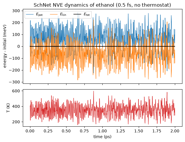
Start from a held-out rMD17 conformation, draw 300 K Maxwell–Boltzmann velocities, and integrate with velocity Verlet at a 0.5 fs time step (the resolution of the paper’s reference trajectories) for 2 ps. No thermostat: in the NVE ensemble any error in the forces shows up directly as drift or noise in the total energy.

import time
from ase import Atoms, units
from ase.md.velocitydistribution import (MaxwellBoltzmannDistribution,
                                         Stationary, ZeroRotation)
from ase.md.verlet import VelocityVerlet

s = load_dataset("rmd17", molecule="ethanol", split="test", n_test=1,
                 quiet=True)[0]
atoms = Atoms(numbers=s["atomic_numbers"], positions=s["pos"])
atoms.calc = calc

MaxwellBoltzmannDistribution(atoms, temperature_K=300)
Stationary(atoms); ZeroRotation(atoms)

DT_FS, N_STEPS = 0.5, 4000                       # 2 ps
dyn = VelocityVerlet(atoms, timestep=DT_FS * units.fs)

t_ps, e_pot, e_kin, temp = [], [], [], []
def record(a=atoms):
    t_ps.append(dyn.nsteps * DT_FS / 1000.0)
    e_pot.append(a.get_potential_energy())
    e_kin.append(a.get_kinetic_energy())
    temp.append(a.get_temperature())
dyn.attach(record, interval=4)

t0 = time.time()
record(); dyn.run(N_STEPS)
print(f"{N_STEPS} NVE steps ({N_STEPS*DT_FS/1000:.1f} ps) "
      f"in {time.time()-t0:.0f}s")

e_pot, e_kin = np.array(e_pot), np.array(e_kin)
e_tot = e_pot + e_kin

4000 NVE steps (2.0 ps) in 113s

2. Total-energy conservation

drift = np.polyfit(t_ps, (e_tot - e_tot[0]) * 1e3, 1)[0]   # meV / ps
print(f"potential-energy fluctuation : {e_pot.std()*1e3:8.2f} meV (the physics)")
print(f"total-energy fluctuation     : {e_tot.std()*1e3:8.3f} meV")
print(f"total-energy drift           : {drift:8.3f} meV/ps")
print(f"conservation ratio  std(E_tot)/std(E_pot) = "
      f"{e_tot.std()/e_pot.std():.4f}")

fig, (a1, a2) = plt.subplots(2, 1, figsize=(6.5, 5), sharex=True,
                             height_ratios=[2, 1])
a1.plot(t_ps, (e_pot - e_pot[0]) * 1e3, label=r"$E_\mathrm{pot}$", lw=0.9)
a1.plot(t_ps, (e_kin - e_kin[0]) * 1e3, label=r"$E_\mathrm{kin}$", lw=0.9)
a1.plot(t_ps, (e_tot - e_tot[0]) * 1e3, "k", label=r"$E_\mathrm{tot}$", lw=1.2)
a1.set_ylabel("energy - initial (meV)")
a1.set_title("SchNet NVE dynamics of ethanol (0.5 fs, no thermostat)")
a1.legend(ncols=3, fontsize=9)
a2.plot(t_ps, temp, lw=0.9, color="tab:red")
a2.set_xlabel("time (ps)"); a2.set_ylabel("T (K)")
fig.tight_layout()
fig.savefig("schnet_nve_energy.png", dpi=110); plt.show()

potential-energy fluctuation :    87.21 meV (the physics)
total-energy fluctuation     :    0.732 meV
total-energy drift           :    0.189 meV/ps
conservation ratio  std(E_tot)/std(E_pot) = 0.0084

Summary

Kinetic and potential energy exchange on the 100 meV scale while the total energy stays flat to well under a meV over 2 ps of thermostat-free dynamics: the autograd forces of the xnn SchNet are conservative to integration accuracy, exactly as eq. 4 of the paper guarantees by construction. Together with schnet_rmd17_train.ipynb (training/accuracy) and examples/fidelity_checks/schnet_verification.ipynb (equation-level fidelity), this completes the SchNet series.