04 · Recreating the MACE architecture, block by block: original MACE and xnn

This tutorial walks through the MACE architecture one block at a time, and for every block builds it twice, once with the original mace-torch (ACEsuit/mace, our ground truth) and once with the xnn re-implementation (xnn.gnn.models.mace), then checks that the two agree to machine precision.

The goal is twofold:

1. Understand MACE. MACE is a message-passing interatomic potential that builds equivariant, many-body atomic features and maps them to an energy. We expose each internal block and its defining equation.

2. Show xnn reproduces MACE exactly. xnn reuses the same maths (real Clebsch–Gordan coupling, learned symmetric contraction) with no mace-torch dependency, only e3nn. By the end we transplant a whole trained-shape MACE from mace-torch into xnn and reproduce its energy and forces to ~1e-15.

Credit. The pedagogy, equations and figures follow the excellent “Deep Dive into the MACE Architecture” developer tutorial by Will Baldwin, based on material by Ilyes Batatia (University of Cambridge). The dual-implementation comparison against xnn is the new contribution here.

References. MACE (NeurIPS 2022) | The Design Space of E(3)-Equivariant Atom-Centred Interatomic Potentials (Multi-ACE) | MACE-OFF | code | docs

0. Setup

This notebook needs the examples extra (installs mace-torch, e3nn, ase, matplotlib, …) on top of xnn:

pip install -e ".[examples]"      # or:  uv sync --extra examples

mace-torch==0.3.16 pins e3nn==0.4.4; xnn runs fine on that pin. We use float64 throughout: MACE’s default, and required for a bit-exact comparison.

import warnings, logging
warnings.filterwarnings("ignore")                     # e3nn/torch.load + TorchScript noise
logging.getLogger("cuequivariance").setLevel(logging.ERROR)

import numpy as np
import torch
torch.set_default_dtype(torch.float64)                # MACE default; needed for exact match
torch.manual_seed(0)

from e3nn import o3
import matplotlib.pyplot as plt
%matplotlib inline

import xnn, mace, e3nn
print("xnn :", xnn.__version__)
print("mace :", mace.__version__, "(original ACEsuit/mace — ground truth)")
print("e3nn :", e3nn.__version__)
print("torch:", torch.__version__, "| CUDA:", torch.cuda.is_available())

xnn : 0.1.0
mace : 0.3.16 (original ACEsuit/mace — ground truth)
e3nn : 0.4.4
torch: 2.5.1+cu121 | CUDA: True

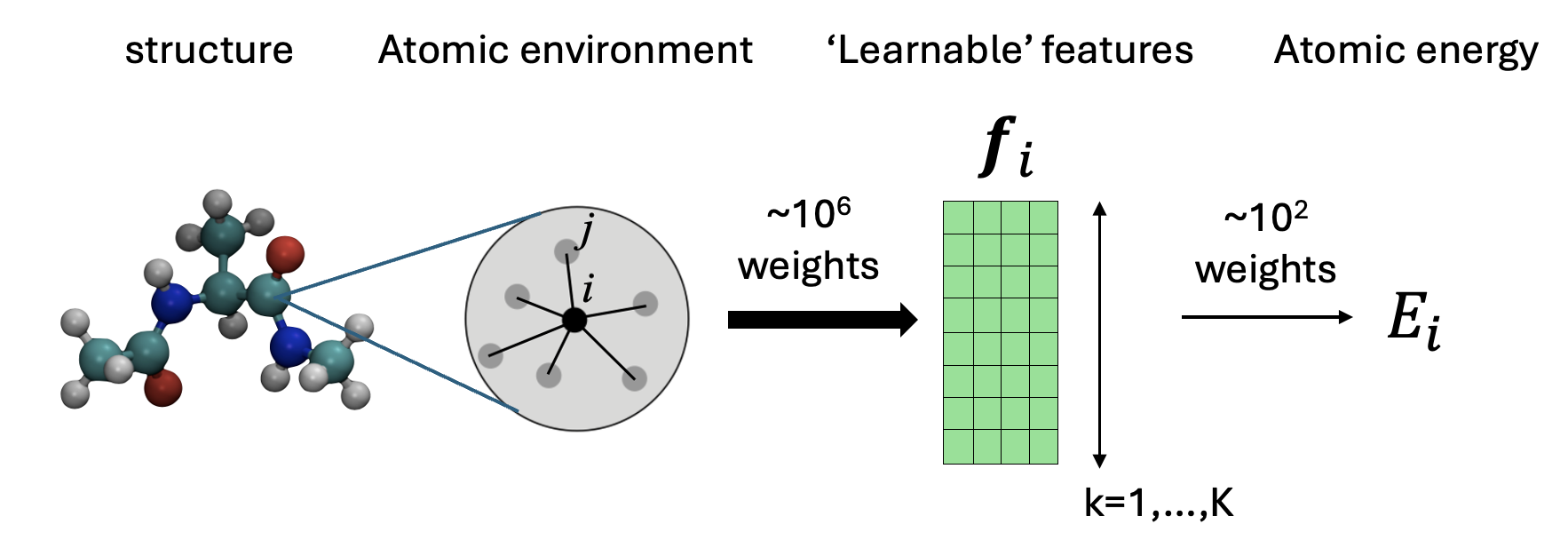
MACE is a function that takes an atomic environment and returns an energy. In classical ML potentials, designing features and fitting are separate steps; in MACE they are blended. As the sketch shows, most of the weights and most of the compute build the atomic features; once you have them, the energy is a relatively simple learnable function of those features.

Below we open up the feature construction and rebuild it, block by block, in both packages.

The MACE architecture at a glance

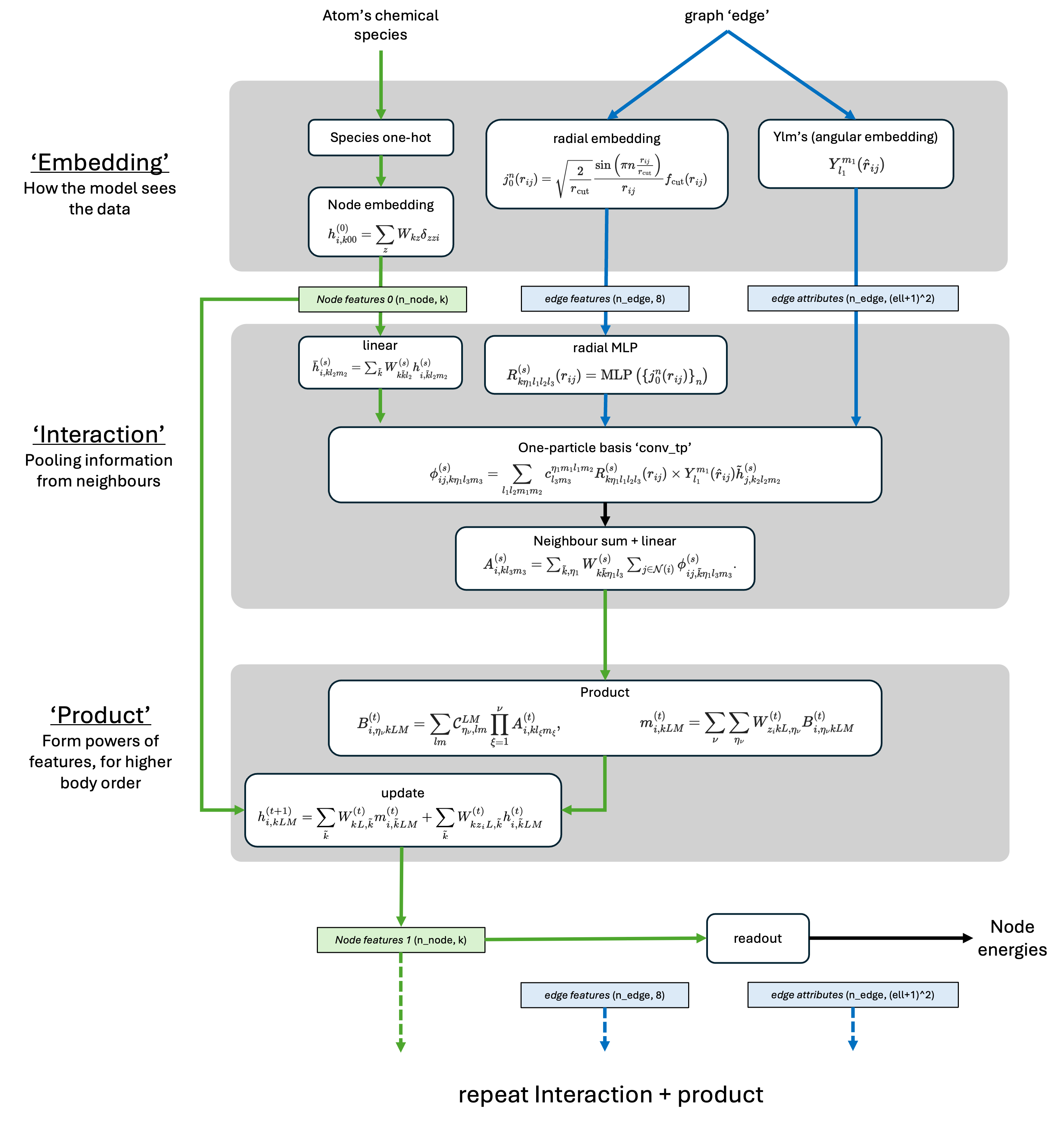
The key steps, repeated for each of \(T\) message-passing layers indexed by \(t = 1, \dots, T\) (num_interactions \(= T\)):

1. Embedding. Turn the structure into initial features: a per-element node feature \(h^{(0)}_i\) for each atom \(i\), plus per-edge length (radial) and direction (spherical harmonic) features.

2. Feature construction.

   • Interaction: pool information from an atom’s neighbours into a 2-body message, the atomic basis \(A_i^{(t)}\).

   • Product: raise \(A_i^{(t)}\) to higher body order via symmetric tensor products, giving the many-body features \(B_i^{(t)}\).

   • Update: mix \(B_i^{(t)}\) (with a self-connection) into the new node features \(h^{(t)}_i\).

3. Readout. Map the invariant part of \(h^{(t)}_i\) to a per-atom site energy \(E_i^{(t)}\).

4. Repeat over layers, then form the total energy by summing every site energy plus a per-element reference energy \(E_0\): $\( E \;=\; \sum_i \Big( E_0(z_i) + \sum_{t=1}^{T} E_i^{(t)} \Big), \qquad \mathbf{F}_i \;=\; -\,\frac{\partial E}{\partial \mathbf{r}_i}. \)$

Symbols used throughout. \(i\): atom index; \(t\): layer index; \(z_i\): chemical element (atomic number) of atom \(i\); \(E_0(z)\): reference energy of an isolated atom of element \(z\); \(\mathbf{r}_i\): position of atom \(i\); \(\mathbf{F}_i\): force on atom \(i\) (obtained by automatic differentiation, so it is exactly the energy gradient).

Default model parameters

We fix one small MACE configuration and build it in both packages. The xnn config funnels through its Config dataclass; the mace-torch model takes the same numbers as keyword arguments. Everything below reuses these two model objects.

from mace import data, modules, tools
import mace.modules as mm
from mace.modules.blocks import RealAgnosticResidualInteractionBlock as MIB

from xnn.common.data import structure_to_graph
from xnn.common.models import build_model, ForceStressOutput
from xnn.common.config import from_dict

# --- shared hyper-parameters ---
SPECIES = [1, 6, 8]            # H, C, O  -> the element channels
CUTOFF  = 3.0                  # r_max (Angstrom)
T       = 2                    # num_interactions (MACE layers)
NCH     = 8                    # num_channels (k)
MAX_ELL = 2                    # l_max of the edge spherical harmonics
MAX_L   = 1                    # l_max kept in the node features between layers
NRBF    = 8                    # number of Bessel radial functions
NPOLY   = 6                    # polynomial-cutoff smoothness
HID     = "8x0e+8x1o"          # hidden_irreps (8 channels of l=0 and l=1)
MLP     = "16x0e"              # final readout MLP width
RMLP    = [64, 64, 64]         # radial MLP hidden sizes (MACE default)
AVG     = 8.0                  # avg_num_neighbors (message normalisation)
CORR    = 3                    # correlation order (body order - 1)
E0      = np.array([-1.0, -3.0, -5.0])   # per-element reference energies

# --- xnn MACE ---
xcfg = from_dict({"model": {"name": "mace", "cutoff": CUTOFF, "n_features": NCH,
    "n_interactions": T, "extra": {"species": SPECIES, "max_ell": MAX_ELL,
    "max_L": MAX_L, "num_channels": NCH, "correlation": CORR, "num_bessel": NRBF,
    "num_polynomial_cutoff": NPOLY, "hidden_irreps": HID, "MLP_irreps": MLP,
    "radial_MLP": RMLP, "avg_num_neighbors": AVG, "atomic_energies": E0.tolist()}}})
xfull  = build_model(xcfg.model)
xmodel = ForceStressOutput(xfull, compute_forces=True).double()   # adds autograd forces

# --- original MACE ---
mmodel = mm.MACE(
    r_max=CUTOFF, num_bessel=NRBF, num_polynomial_cutoff=NPOLY, max_ell=MAX_ELL,
    interaction_cls=MIB, interaction_cls_first=MIB, num_interactions=T,
    num_elements=len(SPECIES), hidden_irreps=o3.Irreps(HID), MLP_irreps=o3.Irreps(MLP),
    atomic_energies=E0, avg_num_neighbors=AVG, atomic_numbers=SPECIES, correlation=CORR,
    gate=torch.nn.functional.silu, radial_MLP=RMLP, radial_type="bessel",
    use_reduced_cg=False, apply_cutoff=True).double()

n_x = sum(p.numel() for p in xfull.parameters())
n_m = sum(p.numel() for p in mmodel.parameters())
print(f"xnn  MACE parameters: {n_x}")
print(f"mace  MACE parameters: {n_m}")

cuequivariance or cuequivariance_torch is not available. Cuequivariance acceleration will be disabled.
xnn  MACE parameters: 25656
mace  MACE parameters: 25456

Copy the weights: mace-torch → xnn

The two models have the same architecture, so we can transplant every weight from mace-torch into xnn. After this, any difference in a block’s output is a genuine implementation difference (not just different random init), so our block-by-block “do they agree?” checks are meaningful.

(The two raw parameter counts differ by a little only because of how each stores the per-element reference energies \(E_0\): xnn uses an embedding table indexed by atomic number, mace-torch a fixed buffer. The trainable network is identical, as the exact energy match at the end confirms.)

The only non-trivial part is the symmetric contraction: xnn stores the per-order weights in a single list weights[0..corr-1] (low → high order), whereas mace-torch keeps the top order in weights_max and the rest in weights (high → low). transplant_sc re-orders them.

def transplant_sc(xsc, msc, corr=CORR):
    # copy mace-torch SymmetricContraction weights into the xnn one
    with torch.no_grad():
        for c in range(len(xsc.contractions)):
            xc, mc = xsc.contractions[c], msc.contractions[c]
            xc.weights[corr - 1].copy_(mc.weights_max)               # top order nu=corr
            for nu in range(1, corr):
                xc.weights[nu - 1].copy_(mc.weights[corr - 1 - nu])  # lower orders

with torch.no_grad():
    xfull.node_embedding.load_state_dict(mmodel.node_embedding.linear.state_dict())
    for i in range(T):
        xfull.interactions[i].load_state_dict(mmodel.interactions[i].state_dict())
        transplant_sc(xfull.products[i].symmetric_contractions,
                      mmodel.products[i].symmetric_contractions, CORR)
        xfull.products[i].linear.load_state_dict(mmodel.products[i].linear.state_dict())
        xr, mr = xfull.readouts[i], mmodel.readouts[i]
        if "NonLinear" in type(mr).__name__:
            xr.linear_1.load_state_dict(mr.linear_1.state_dict())
            xr.linear_2.load_state_dict(mr.linear_2.state_dict())
        else:
            xr.linear.load_state_dict(mr.linear.state_dict())
    for z, e in zip(SPECIES, E0):
        xfull.atom_ref.weight[z] = float(e)                          # reference energies

# a small helper for the agreement checks below
def report(name, diff, tol=1e-10):
    tag = "OK " if diff <= tol else "!! "
    print(f"{tag}{name:<42} max|xnn - mace| = {diff:.2e}")

print("weights transplanted: mace-torch -> xnn")

weights transplanted: mace-torch -> xnn

Spherical tensors and e3nn: the shared language

Both MACE and xnn represent directional information as spherical tensors and manipulate them with e3nn. The core fact: when you rotate a direction \(\mathbf{r}\to R\mathbf{r}\), the spherical harmonics \(Y_l^m\) transform in a known, linear way,

\[ Y_l^m(R\,\mathbf{r}) \;=\; \sum_{m'=-l}^{l} D^l_{mm'}(R)\; Y_l^{m'}(\mathbf{r}). \]

Symbols. \(\mathbf{r}\): a 3D direction vector; \(R\): a \(3\times3\) rotation matrix; \(l = 0, 1, 2, \dots\): the degree (angular frequency) of the harmonic; \(m = -l, \dots, +l\): the order (there are \(2l+1\) values of \(m\) for each \(l\)); \(Y_l^m(\mathbf{r})\): the real spherical harmonic of degree \(l\), order \(m\); \(D^l_{mm'}(R)\): the Wigner D-matrix, the \((2l+1)\times(2l+1)\) matrix that mixes the order-\(m\) components among themselves under the rotation \(R\).

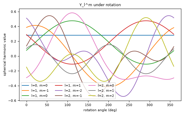
The key consequence: a rotation only mixes components within the same degree \(l\), and never mixes different \(l\)’s. So the \(l=0\) part (\(D^0 = 1\)) is left completely unchanged; it is rotation-invariant. That is how we can always recover an invariant quantity when we need one. Let’s evaluate \(Y_l^m\) for \(l = 0, 1, 2\) on one vector.

spherical_harmonics = o3.SphericalHarmonics([0, 1, 2], normalize=True)
vector = torch.tensor([1.0, 0.2, 0.75])
print(spherical_harmonics(vector))

tensor([ 0.2821,  0.3860,  0.0772,  0.2895,  0.5113,  0.1364, -0.2918,  0.1023,
        -0.1491])

The array has 9 elements: \(l=0\) (1 value), \(l=1\) (3 values), \(l=2\) (5 values), concatenated as $\([\,Y_0^0,\ \ Y_1^{-1}, Y_1^{0}, Y_1^{1},\ \ Y_2^{-2}, Y_2^{-1}, Y_2^{0}, Y_2^{1}, Y_2^{2}\,].\)\( This \)(l,m)$-flattened layout is how MACE (and xnn) store all equivariant arrays.

Now rotate the vector through a full turn and watch each component: the \(l=0\) piece is constant (invariant), while higher-\(l\) pieces oscillate faster.

from scipy.spatial.transform import Rotation
axis = np.array([0, 0.7071, 0.7071])
vec  = np.array([1.0, 0.2, 0.75])
rots = [Rotation.from_rotvec(i * 2*np.pi * axis / 360).as_matrix() @ vec for i in range(360)]
vals = spherical_harmonics(torch.tensor(np.array(rots)))

labels = [f"l={l}, m={m}" for l in range(3) for m in range(-l, l+1)]
plt.figure(figsize=(7, 4))
plt.plot(vals.numpy(), label=labels)
plt.legend(ncol=3, fontsize=8); plt.xlabel("rotation angle (deg)")
plt.ylabel("spherical harmonic value"); plt.title("Y_l^m under rotation"); plt.show()

Invariants that actually carry angular information

Just taking the \(l=0\) piece of a single direction is uninformative (it is the same constant for every direction). To build a descriptive invariant we combine two spherical tensors with a tensor product \(\otimes\), which e3nn performs while correctly tracking all the \((l,m)\) bookkeeping:

\[ \big[A_l^m\big] \;\otimes\; \big[B_l^m\big] \;=\; \big[C_L^M\big]. \]

Symbols. \(A_l^m\) and \(B_l^m\): the two input spherical tensors (each a full set of \((l,m)\) components, e.g. the spherical harmonics of two directions); \(C_L^M\): the output spherical tensor, indexed by its own degree \(L\) and order \(M\). Internally the product of an input degree-\(l_1\) part with an input degree-\(l_2\) part is re-coupled (using Clebsch–Gordan coefficients) into outputs whose degrees \(L\) range over \(|l_1-l_2|,\dots,l_1+l_2\).

Because \(C\) is itself a spherical tensor, its \(L=0\) part is again rotation-invariant; but, unlike the raw \(l=0\) inputs, it now depends on the angle between \(A\) and \(B\). This tensor product is the fundamental operation MACE is built on. Below we set up a product of two \((l=0,1,2)\) tensors that outputs three invariant (\(L=0\)) numbers.

# a tensor product of two (l=0,1,2) arrays -> three invariant (l=0) outputs
tp = o3.FullyConnectedTensorProduct(
    o3.Irreps("1x0e+1x1o+1x2e"), o3.Irreps("1x0e+1x1o+1x2e"),
    o3.Irreps("3x0e"), internal_weights=False)
print(tp)
try:
    tp.visualize()                       # schematic of how inputs combine into outputs
except AttributeError:
    print("(skipping tp.visualize(): needs older matplotlib than this environment)")

FullyConnectedTensorProduct(1x0e+1x1o+1x2e x 1x0e+1x1o+1x2e -> 3x0e | 9 paths | 9 weights)
(skipping tp.visualize(): needs older matplotlib than this environment)

np.random.seed(0)
v1 = np.random.randn(3); v1 /= np.linalg.norm(v1)
v2 = np.random.randn(3); v2 /= np.linalg.norm(v2)
w  = torch.arange(1, 10, 1, dtype=torch.float64)      # fixed weights, for illustration

def invariants(a, b):
    return tp(spherical_harmonics(torch.tensor(a)).unsqueeze(0),
              spherical_harmonics(torch.tensor(b)).unsqueeze(0), weight=w)

print("invariants          :", invariants(v1, v2).detach().numpy())

# rotate BOTH vectors by the same rotation -> invariants unchanged
R = Rotation.from_rotvec(77.7 * 2*np.pi * axis / 360).as_matrix()
print("invariants (rotated):", invariants(R @ v1, R @ v2).detach().numpy())

invariants          : [[0.25239444 0.34801136 0.44362828]]
invariants (rotated): [[0.25239444 0.34801136 0.44362828]]

The two rows match: the outputs are invariant to rotating the whole system, yet (try changing the seed) they do change when the angle between the vectors changes. That is exactly the property MACE needs.

Recreating MACE feature construction, block by block

We now feed a real molecule (ethanol, C₂H₆O; it has exactly our H/C/O elements) through the model and inspect each block, comparing xnn against mace-torch at every step.

0. Data prep: structure → atoms + edges

MACE represents a structure as a list of atoms plus edges (pairs of atoms within r_max). mace-torch uses AtomicData; xnn uses AtomicGraph via structure_to_graph. Both build the same neighbour list.

from mace.tools import AtomicNumberTable, torch_geometric
from mace.data import AtomicData, Configuration
from ase.build import molecule

atoms = molecule("CH3CH2OH")                       # ethanol: 2 C, 1 O, 6 H
Z   = atoms.get_atomic_numbers()                   # (n_atoms,)
pos = atoms.get_positions()                        # (n_atoms, 3)

# --- xnn ---
graph = structure_to_graph({"pos": pos, "atomic_numbers": Z}, CUTOFF)

# --- original mace ---
zt   = AtomicNumberTable(SPECIES)
conf = Configuration(atomic_numbers=Z, positions=pos, properties={}, property_weights={})
ad   = AtomicData.from_config(conf, z_table=zt, cutoff=CUTOFF)
mbatch = next(iter(torch_geometric.dataloader.DataLoader([ad], batch_size=1)))

print("elements       :", Z.tolist())
print("xnn  nodes/edges:", graph.num_nodes, "/", graph.num_edges)
print("mace  nodes/edges:", mbatch.node_attrs.shape[0], "/", mbatch.edge_index.shape[1])
print("node_attrs (one-hot over [H,C,O]), first 3 atoms:\n",
      xfull.node_attr(graph.atomic_numbers)[:3].int().numpy())

elements       : [6, 6, 8, 1, 1, 1, 1, 1, 1]
xnn  nodes/edges: 9 / 58
mace  nodes/edges: 9 / 58
node_attrs (one-hot over [H,C,O]), first 3 atoms:
 [[0 1 0]
 [0 1 0]
 [0 0 1]]

node_attrs is a one-hot over the element set: [1,0,0]=H, [0,1,0]=C, [0,0,1]=O. Edges are stored as edge_index = [senders; receivers]. From these we get each edge’s length and direction (both packages agree; xnn uses the convention \(\mathbf{r}_{ij} = \mathbf{r}_{\text{dst}} - \mathbf{r}_{\text{src}}\)).

# edge vectors & lengths
vectors, lengths = modules.utils.get_edge_vectors_and_lengths(
    positions=mbatch["positions"], edge_index=mbatch["edge_index"], shifts=mbatch["shifts"])
print("mace  vectors/lengths:", tuple(vectors.shape), tuple(lengths.shape))
print("xnn  edge_vectors   :", tuple(graph.edge_vectors().shape))

mace  vectors/lengths: (58, 3) (58, 1)
xnn  edge_vectors   : (58, 3)

1. Embeddings

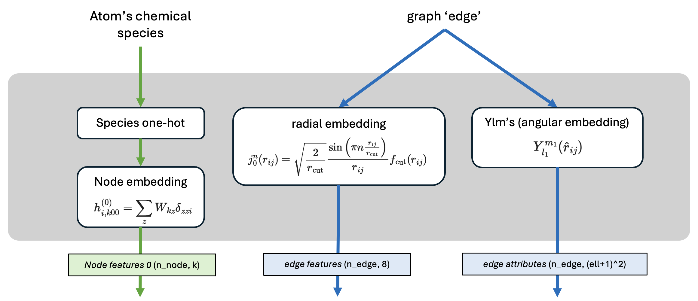
Node embedding. Each atom \(i\) is given a length-\(K\) feature vector that depends only on its chemical element:

\[ h^{(0)}_{i,k00} \;=\; \sum_{z} W_{kz}\,\delta_{z\, z_i}. \]

Here,

• \(h^{(0)}_{i,k00}\): the initial (\(t=0\)) feature of atom \(i\) in channel \(k\); the trailing subscripts 00 mean degree \(l=0\), order \(m=0\) (these features are pure scalars/invariants).

• \(k = 1, \dots, K\): the channel index; \(K\) (num_channels) is the fundamental descriptor width.

• \(z\): runs over the chemical elements. Thus, \(z_i\) the element of atom \(i\)

• \(\delta_{z\,z_i}\): the Kronecker delta (1 if \(z = z_i\), else 0), so the sum just selects the column of \(W\) for atom \(i\)’s element

• \(W_{kz}\): the learnable embedding weights.

In code, \(\delta_{z\,z_i}\) is the one-hot node_attrs and \(W\) is a linear layer.

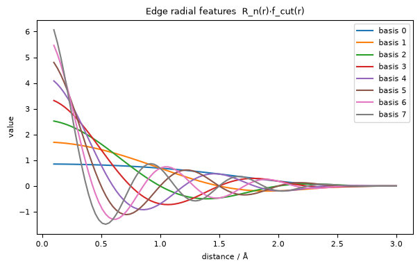
Edge embedding. Each edge \(i\!-\!j\) contributes two things: its length \(r_{ij} = \lVert \mathbf{r}_{ij}\rVert\) is expanded in Bessel radial functions multiplied by a smooth polynomial cutoff \(f_{\rm cut}\) (an invariant feature), and its direction \(\hat{\mathbf r}_{ij} = \mathbf{r}_{ij}/r_{ij}\) is turned into spherical harmonics \(Y_l^m(\hat{\mathbf r}_{ij})\) (an equivariant feature).

We compute all three embeddings in both packages and check they match. (Because the two neighbour lists can order edges differently, we compare the spherical harmonics on a shared set of edge vectors; see the code comment.)

# --- node embedding:  h0[i,k] = sum_z W[k,z] * delta(z, z_i) ---
na  = xfull.node_attr(graph.atomic_numbers)           # delta_{z z_i}: one-hot over [H,C,O], shape (N, 3)
h0x = xfull.node_embedding(na)                        # W @ delta  ->  (N, K=8) initial scalar features
h0m = mmodel.node_embedding(mbatch["node_attrs"])
report("node embedding  h^(0)", (h0x - h0m).abs().max().item())

# --- edge radial embedding ---
edge = xfull.edge_feat(graph)                        # dict: edge_sh, edge_radial, edge_length, edge_vec
mr, _ = mmodel.radial_embedding(lengths, mbatch["node_attrs"], mbatch["edge_index"], zt.zs)
report("radial embedding  R_n(r)*f_cut(r)", (edge["edge_radial"] - mr).abs().max().item())

# --- edge spherical harmonics (compare on the SAME vectors) ---
ir_sh  = o3.Irreps.spherical_harmonics(MAX_ELL)      # 1x0e+1x1o+1x2e
sh_x   = o3.spherical_harmonics(ir_sh, graph.edge_vectors(), normalize=True, normalization="component")
sh_m   = mmodel.spherical_harmonics(graph.edge_vectors())
report("spherical harmonics  Y_l^m", (sh_x - sh_m).abs().max().item())

print("\nshapes:  h0", tuple(h0x.shape),
      " edge_radial", tuple(edge["edge_radial"].shape),
      " edge_sh", tuple(edge["edge_sh"].shape))

OK node embedding  h^(0)                      max|xnn - mace| = 0.00e+00
OK radial embedding  R_n(r)*f_cut(r)          max|xnn - mace| = 1.25e-15
OK spherical harmonics  Y_l^m                 max|xnn - mace| = 0.00e+00

shapes:  h0 (9, 8)  edge_radial (58, 8)  edge_sh (58, 9)

The learnable-free part of the radial embedding (Bessel × cutoff) looks like this:

dists = torch.linspace(0.1, CUTOFF, 100).unsqueeze(-1)
radials, _ = mmodel.radial_embedding(dists, None, None, None)
plt.figure(figsize=(7, 4))
for i in range(radials.shape[1]):
    plt.plot(dists.squeeze(), radials[:, i].detach(), label=f"basis {i}")
plt.title("Edge radial features  R_n(r)·f_cut(r)")
plt.xlabel("distance / Å"); plt.ylabel("value"); plt.legend(fontsize=8); plt.show()

2. Interaction: pooling over neighbours

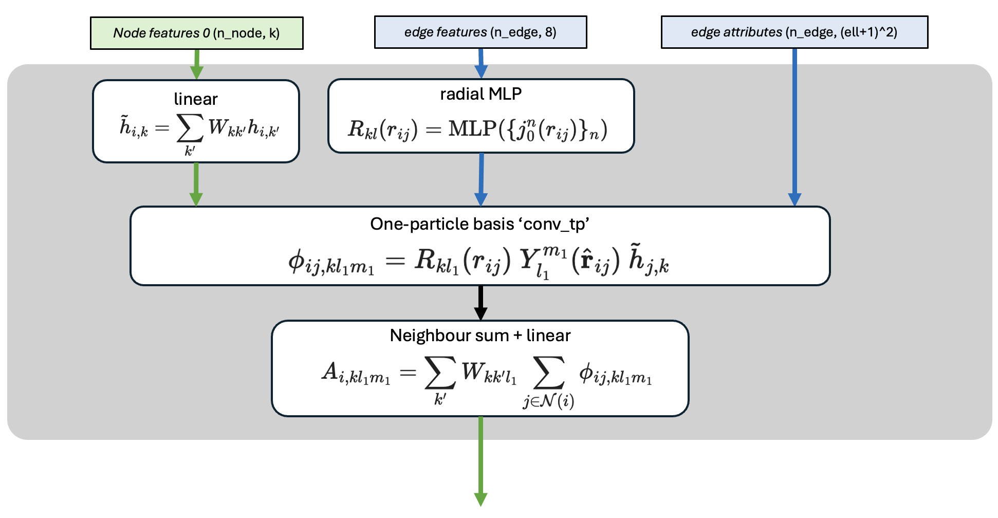
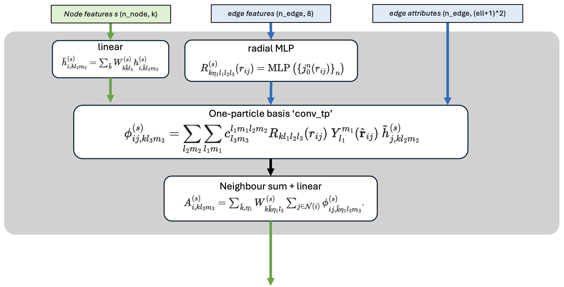
The interaction pools information from an atom’s neighbours into a 2-body atomic basis \(A_{i,klm}^{(t)}\), while tracking every array’s \((l,m)\) indices. Schematically, for atom \(i\) at layer \(t\):

\[ A_{i,klm}^{(t)} \;=\; \sum_{j \,\in\, \mathcal{N}(i)} R_{kl}(r_{ij})\;\, Y_l^m(\hat{\mathbf r}_{ij})\;\, h^{(t-1)}_{j,k}, \]

pooled (summed) over the neighbours and then normalised by avg_num_neighbors.

Symbols. \(\mathcal{N}(i)\): the neighbours \(j\) of atom \(i\) within the cutoff; \(h^{(t-1)}_{j,k}\): the (previous-layer) features of neighbour \(j\) in channel \(k\); \(Y_l^m(\hat{\mathbf r}_{ij})\): spherical harmonics of the edge direction; \(R_{kl}(r_{ij})\): a learnable radial function, one per channel–degree pair \((k,l)\), produced by passing the Bessel edge features through a small MLP (the radial MLP). The product \(R_{kl}\,Y_l^m\) is exactly the weighted tensor product of §”Spherical tensors”, so \(A\) stays a proper spherical tensor. It is called 2-body because each term involves atom \(i\) and a single neighbour \(j\).

We run mace-torch’s and xnn’s interaction blocks on the same embeddings and compare the resulting atomic basis \(A\) and the residual self-connection \(sc\) (a learnable shortcut of the atom’s own features, added back later in the product block).

xI, mI = xfull.interactions[0], mmodel.interactions[0]

xA, xsc = xI(na, h0x, edge["edge_sh"], edge["edge_radial"], graph.edge_index)
mA, msc = mI(node_attrs=na, node_feats=h0x, edge_attrs=edge["edge_sh"],
             edge_feats=edge["edge_radial"], edge_index=graph.edge_index, cutoff=None)

report("interaction message  A", (xA - mA).abs().max().item())
report("residual self-connection  sc", (xsc - msc).abs().max().item())
print("A shape (atoms, channels, dim SH):", tuple(xA.shape))

OK interaction message  A                     max|xnn - mace| = 0.00e+00
OK residual self-connection  sc               max|xnn - mace| = 0.00e+00
A shape (atoms, channels, dim SH): (9, 8, 9)

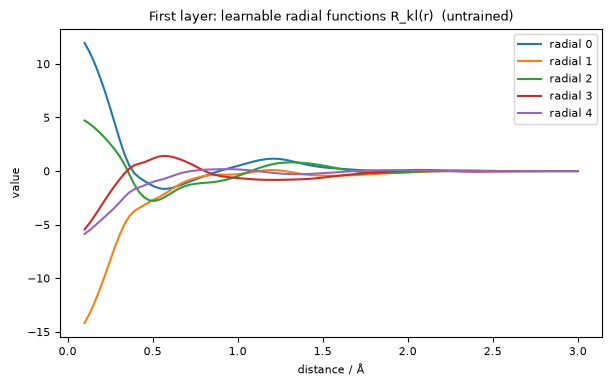
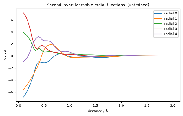
We can visualise the learnable radial functions: the output of the radial MLP, one function of distance per tensor-product weight. Untrained they are just smooth random curves; training shapes them.

ef, _ = mmodel.radial_embedding(dists, None, None, None)
tp_w = mmodel.interactions[0].conv_tp_weights(ef).detach()
plt.figure(figsize=(7, 4))
for i in range(5):
    plt.plot(dists.squeeze(), tp_w[:, i], label=f"radial {i}")
plt.title("First layer: learnable radial functions R_kl(r)  (untrained)")
plt.xlabel("distance / Å"); plt.ylabel("value"); plt.legend(fontsize=8); plt.show()

3. Product: building many-body features

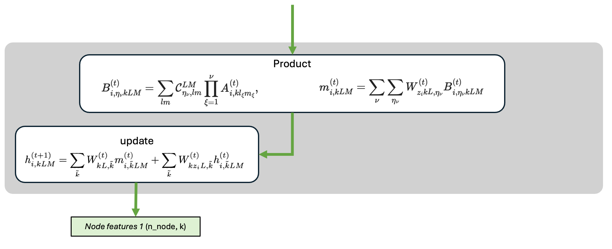
This is the heart of MACE. The product block raises the body order of the features by multiplying \(\nu\) copies of the atomic basis \(A\) together and re-coupling them into a proper spherical tensor with generalised Clebsch–Gordan coefficients:

\[ B^{(t)}_{i,\eta_\nu k L M} \;=\; \sum_{l_1 m_1}\cdots\sum_{l_\nu m_\nu} \mathcal{C}^{L M}_{\eta_\nu,\, l_1 m_1 \dots l_\nu m_\nu}\; \prod_{\xi=1}^{\nu} A^{(t)}_{i,\,k\, l_\xi m_\xi}. \]

Symbols. \(A^{(t)}_{i,klm}\): the 2-body atomic basis from the interaction (atom \(i\), channel \(k\), degree \(l\), order \(m\)); \(\nu\): the correlation order (correlation), i.e. how many copies of \(A\) are multiplied together (the resulting feature is \((\nu+1)\)-body); \(\xi = 1,\dots,\nu\): the product index over those copies, each with its own degree/order \((l_\xi, m_\xi)\); \(L, M\): the degree and order of the output feature \(B\); \(\mathcal{C}^{LM}_{\eta_\nu, \dots}\): the generalised Clebsch–Gordan coefficients (the “\(U\) tensors”) that combine the \(\nu\) inputs into something that transforms like a single degree-\(L\) object; \(\eta_\nu\): an index enumerating the distinct symmetric coupling paths that yield the same output \((L,M)\); \(B^{(t)}_{i,\eta_\nu kLM}\): the resulting many-body feature. A final linear layer mixes the paths \(\eta_\nu\) and channels \(k\), and the self-connection \(sc\) is added, producing the updated node features \(h^{(t)}_i\).

xnn implements the same learned symmetric contraction as mace-torch: its Clebsch–Gordan \(U\) basis is bit-identical and the contraction reproduces mace-torch to ~1e-16 given the same weights (verified in tests/test_mace.py). This is precisely the piece the old xnn MACE only approximated (with a plain TensorSquare).

# symmetric contraction of A (nu copies) + linear mix + self-connection sc  ->  h^(1)
xB = xfull.products[0](xA, xsc, na)                    # args: (atomic basis A, self-connection sc, node_attrs)
mB = mmodel.products[0](node_feats=mA, node_attrs=na, sc=msc)
report("product + update  h^(1)", (xB - mB).abs().max().item())
# last dim = (max_L + 1)^2 * num_channels = (1+1)^2 * 8 = 4 * 8 = 32
print("h^(1) shape (atoms, (max_L+1)^2 · channels):", tuple(xB.shape), "= (N, 4·8)")

OK product + update  h^(1)                    max|xnn - mace| = 0.00e+00
h^(1) shape (atoms, (max_L+1)^2 · channels): (9, 32) = (N, 4·8)

The last dimension is \(32 = 8 \times 4\): 8 channels times the 4 components of the retained \(l=0\) and \(l=1\) features. Whether higher-\(l\) (equivariant) features are kept between layers is set by max_L (here max_L=1). The first 8 values (the \(l=0\) part) are invariant; the rest are equivariant and rotate with the molecule.

4. Readout: features → site energy

The readout maps the invariant (\(l=0\)) part of the node features to a per-atom site-energy contribution. Early layers use a simple linear map; the final layer uses a small gated MLP:

\[\begin{split} \mathcal{R}^{(t)}\!\left(h_i^{(t)}\right) \;=\; \begin{cases} \displaystyle\sum_{k} W_k^{(t)}\, h^{(t)}_{i,k00} & \text{if } t < T, \\[10pt] \mathrm{MLP}\!\left(\{\, h^{(t)}_{i,k00} \,\}_k\right) & \text{if } t = T. \end{cases} \end{split}\]

Symbols. \(\mathcal{R}^{(t)}\): the readout at layer \(t\); \(T\): the total number of layers (num_interactions); \(h^{(t)}_{i,k00}\): the invariant (degree \(l=0\)) part of atom \(i\)’s features in channel \(k\) (only the scalar part enters, so the site energy is rotation-invariant); \(W_k^{(t)}\): learnable linear weights; \(\mathrm{MLP}\): a one-hidden-layer perceptron with a SiLU gate (gate), used only at the last layer. The output is \(E_i^{(t)}\), the layer-\(t\) site-energy contribution of atom \(i\).

xe = xfull.readouts[0](xB).squeeze(-1)
me = mmodel.readouts[0](mB).squeeze(-1)
report("layer-0 readout (site energy)", (xe - me).abs().max().item())
print("per-atom energy contribution (layer 0):\n", xe.detach().numpy())

OK layer-0 readout (site energy)              max|xnn - mace| = 0.00e+00
per-atom energy contribution (layer 0):
 [0.34936828 0.33550752 0.41893127 0.33609633 0.3555528  0.3555528
 0.37259495 0.37439018 0.37439018]

5. Repeat: the whole model, end to end

Interaction → product → readout repeats for each layer, and all site energies are summed together with the per-element reference \(E_0\) to give the total energy; forces are its gradient w.r.t. positions. Here we let each package run its own full data pipeline and forward pass independently, then compare: the real end-to-end test.

# xnn: graph -> energy + forces
ox  = xmodel(graph)
E_x = float(ox["energy"]); F_x = ox["forces"].detach().numpy()

# mace: its own batch -> energy + forces
om  = mmodel(mbatch.to_dict(), compute_force=True)
E_m = float(om["energy"]); F_m = om["forces"].detach().numpy()

print(f"total energy   xnn = {E_x:.10f} eV")
print(f"total energy   mace = {E_m:.10f} eV\n")
report("FULL MODEL  total energy", abs(E_x - E_m))
report("FULL MODEL  per-atom forces", np.abs(F_x - F_m).max())

total energy   xnn = -14.6911114202 eV
total energy   mace = -14.6911114202 eV

OK FULL MODEL  total energy                   max|xnn - mace| = 1.78e-15
OK FULL MODEL  per-atom forces                max|xnn - mace| = 5.69e-16

Energy and forces agree to ~1e-15: xnn reproduces mace-torch to machine precision, using only e3nn. That is the whole point: the same physics, re-expressed on the xnn abstractions (AtomicGraph, featurizers, ForceStressOutput).

The interaction block in more detail (second layer)

At the second layer the interaction is harder, because the incoming node features are no longer just scalars; they carry \((l,m)\) indices (we kept max_L=1). The learnable radial functions now feed a richer tensor product, so the radial MLP must output more weights than in the first layer. We can see this directly:

for layer in (0, 1):
    n_w = mmodel.interactions[layer].conv_tp_weights(ef).shape[1]
    print(f"layer {layer}: radial MLP outputs {n_w} tensor-product weights")

# the layer-1 learnable radials
tp_w1 = mmodel.interactions[1].conv_tp_weights(ef).detach()
plt.figure(figsize=(7, 4))
for i in range(5):
    plt.plot(dists.squeeze(), tp_w1[:, i], label=f"radial {i}")
plt.title("Second layer: learnable radial functions  (untrained)")
plt.xlabel("distance / Å"); plt.ylabel("value"); plt.legend(fontsize=8); plt.show()

layer 0: radial MLP outputs 24 tensor-product weights
layer 1: radial MLP outputs 56 tensor-product weights

xnn bonus. In the original MACE num_interactions is fixed to 2; in xnn it is fully flexible, T = 0 … N. T = 0 is a pure \(E_0\) / pair-repulsion baseline, and any T ≥ 1 stacks the interaction/product/readout above exactly as shown here.

Summary

We rebuilt MACE block by block in both the original mace-torch and xnn, and verified agreement at every stage:

block	equation	max|xnn − mace|
node embedding	\(h^{(0)} = W\,\theta\)	0
radial embedding	\(R_n(r)\,f_{\rm cut}(r)\)	~1e-15
spherical harmonics	\(Y_l^m(\hat r_{ij})\)	~1e-15
interaction	2-body message \(A\)	~1e-16
product	symmetric contraction \(B\)	~1e-16
readout	site energy	~1e-16
full model	energy & forces	~1e-15

xnn reuses the same equivariant maths as MACE (real Clebsch–Gordan coupling, learned symmetric contraction) with no mace-torch dependency (only e3nn) and slots it into the shared xnn abstractions so data loading, autograd forces/stress, training, and ASE/LAMMPS deployment are identical across every model in the package.

Where next.

• ../../fidelity_checks/mace_verification.ipynb: the same comparison at the level of individual e3nn blocks and the Clebsch–Gordan U tensors.

• mace_argon_train_test.ipynb: a full train/test pipeline, xnn vs mace-torch.

• mace_argon_density_md.ipynb: liquid-Argon density from NPT MD.