
Training & testing NequIP on Argon MD data: xnn vs the original NequIP, step by step#
This notebook runs a complete end-to-end interatomic-potential pipeline on a
realistic Argon dataset, twice, once with the xnn NequIP
(xnn.gnn.models.nequip) and once with the original nequip package
(mir-group/nequip), and compares the two at every stage:
stage |
xnn |
original NequIP |
comparison |
|---|---|---|---|
1. data → graphs |
|
|
#edges, \(\langle\)neighbours\(\rangle\) |
2. model build |
|
|
parameter count |
3. identical function? |
n/a |
n/a |
weight transplant → same E, F |
4. training |
|
native training loop |
loss curves, time |
5. test evaluation |
autograd forces |
autograd forces |
energy/force RMSE & MAE |
Both models use identical hyper-parameters, the same train/validation split, the
same loss (per-atom energy MSE + force MSE) and the same optimiser/schedule, so
the only thing that differs is the implementation. The data
(../../../datasets/argon_md/argon_{train,test}.xyz, shared across the examples) carries
REF_energy, REF_forces, REF_stress.
The companion notebook
../../fidelity_checks/nequip_verification.ipynbproves the two implementations are the same function block-by-block to machine precision; here we confirm it on the actual Argon data and then show the full training/testing pipeline gives matching results.
0. Setup#
float32 on the GPU for training speed (both models identically).
# silence the expected warnings
import logging
import warnings

logging.disable(logging.WARNING)                     # nequip's torch-version notice
warnings.filterwarnings("ignore", category=UserWarning)
warnings.filterwarnings(
    "ignore",
    category=FutureWarning,
    message="You are using `torch.load` with `weights_only=False`",
)

import time
import numpy as np
import torch
import matplotlib.pyplot as plt
import ase.io

torch.set_default_dtype(torch.float32)
torch.manual_seed(0)

DEVICE = "cuda" if torch.cuda.is_available() else "cpu"
DATA = "../../../datasets/argon_md"                                # shared across the examples
import xnn, nequip
print("xnn:", xnn.__version__, "| nequip (original):", nequip.__version__)
print("device:", DEVICE, "|", torch.cuda.get_device_name(0) if DEVICE == "cuda" else "")
xnn: 0.1.0 | nequip (original): 0.6.2
device: cuda | NVIDIA A100 80GB PCIe
1. Load the data and the reference energy \(E_0\)#
The first training frame is an isolated atom (config_type=IsolatedAtom),
fixing the per-element reference energy \(E_{0,\mathrm{Ar}}\): in NequIP language,
the per-species shift per_species_rescale_shifts (the per-species scale is
left at 1). The MD coordinates are unwrapped, so we wrap() each frame into its
cell before building neighbour lists (physically identical under PBC). This shared
list of structures feeds both pipelines.
from xnn.common.data import load_dataset
E0 = {18: 0.0}   # argon isolated-atom reference energy
train_structs = load_dataset("argon_md", split="train")
test_structs = load_dataset("argon_md", split="test")
SPECIES = sorted({int(z) for s in train_structs for z in s["atomic_numbers"]})
CUTOFF = 6.0
print(f"train: {len(train_structs)}  test: {len(test_structs)}  species: {SPECIES}  E0: {E0}")
train: 200 test: 50 species: [18] E0: {18: 0.0}
Quick EDA#
epa = np.array([s["energy"]/len(s["atomic_numbers"]) for s in train_structs])
cellL = np.array([np.diag(s["cell"]).mean() for s in train_structs])
fig, ax = plt.subplots(1, 2, figsize=(9, 3.0))
ax[0].hist(epa, bins=30); ax[0].set_xlabel("energy/atom [eV]"); ax[0].set_title("per-atom energy")
ax[1].hist(cellL, bins=30); ax[1].set_xlabel("mean cell length [Å]"); ax[1].set_title("box size")
plt.tight_layout(); plt.show()
print(f"E/atom {epa.min():.3f}..{epa.max():.3f} eV ; cell {cellL.min():.1f}..{cellL.max():.1f} Å")
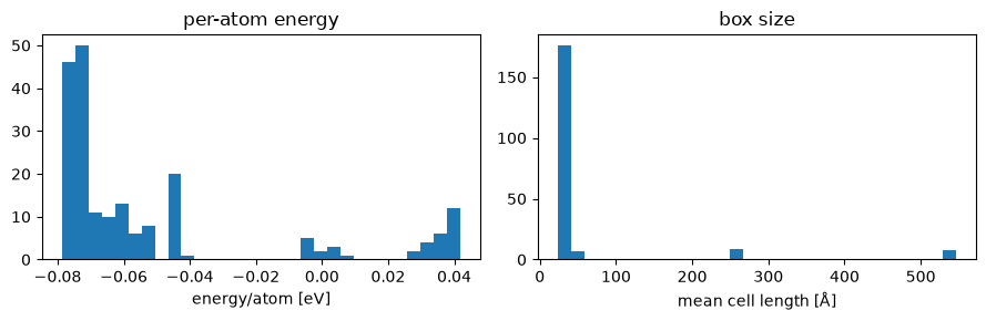
E/atom -0.079..0.042 eV ; cell 23.2..546.4 Å
2. Build graphs: xnn and original NequIP data pipelines#
We construct the dataset with each code’s own neighbour-list machinery and compare
the resulting graphs and the average number of neighbours \(\lambda\), which NequIP
uses to normalise messages by \(1/\sqrt{\lambda}\) (avg_num_neighbors).
One data quirk first: the Argon set contains a few fully vaporised snapshots
(546 Å boxes) in which no pair of atoms is within the 6 Å cutoff. xnn (like
MACE) tolerates edgeless graphs (a local model simply predicts \(\sum_i E_{0,z_i}\)
for them), but the original nequip data pipeline raises on such frames.
Since they carry no learnable signal for a local potential either way, we drop
them from both pipelines so the two models see exactly the same data
(7 of 200 train frames, 2 of 50 test frames).
from xnn.common.data import AtomicDataset
from nequip.data import AtomicData, AtomicDataDict
from nequip.data.dataloader import DataLoader as NequipDataLoader
from nequip.data.transforms import TypeMapper

# --- drop the edgeless (fully vaporised) frames from both pipelines ---
def with_edges(structs):
    ds = AtomicDataset(structs, CUTOFF)
    keep = [i for i in range(len(structs)) if ds[i].num_edges > 0]
    return [structs[i] for i in keep], len(structs) - len(keep)

train_structs, n_drop_tr = with_edges(train_structs)
test_structs,  n_drop_te = with_edges(test_structs)
print(f"dropped edgeless frames: train {n_drop_tr}, test {n_drop_te} "
      "(nequip's pipeline rejects them; zero signal for a local model)")

# --- xnn graphs ---
xnn_train = AtomicDataset(train_structs, CUTOFF)
xnn_test  = AtomicDataset(test_structs,  CUTOFF)
xnn_edges = np.array([xnn_train[i].num_edges for i in range(len(xnn_train))])
xnn_atoms = np.array([xnn_train[i].num_nodes for i in range(len(xnn_train))])
LAMBDA = float(xnn_edges.sum() / xnn_atoms.sum())

# --- original NequIP graphs ---
TM = TypeMapper(chemical_symbols=["Ar"])
def to_nequip(structs):
    out = []
    for s in structs:
        d = AtomicData.from_points(
            pos=torch.tensor(s["pos"], dtype=torch.get_default_dtype()),
            r_max=CUTOFF,
            atomic_numbers=torch.tensor(s["atomic_numbers"]),
            cell=torch.tensor(s["cell"], dtype=torch.get_default_dtype()),
            pbc=torch.tensor([True, True, True]),
            total_energy=torch.tensor([s["energy"]], dtype=torch.get_default_dtype()),
            forces=torch.tensor(s["forces"], dtype=torch.get_default_dtype()))
        out.append(TM(d))
    return out
nequip_train = to_nequip(train_structs)
nequip_test  = to_nequip(test_structs)
nequip_edges = np.array([d.edge_index.shape[1] for d in nequip_train])

print(f"total edges     xnn = {int(xnn_edges.sum()):>8d}   nequip = {int(nequip_edges.sum()):>8d}")
print(f"per-frame edges max|xnn - nequip| = {np.abs(xnn_edges - nequip_edges).max()}"
      "  (identical neighbour lists)")
print(f"avg neighbours (edges/atom):  lambda = {LAMBDA:.3f}")
print(f"--> using avg_num_neighbors = {LAMBDA:.3f} for both models "
      "(upstream 'auto' computes the same statistic)")
dropped edgeless frames: train 7, test 2 (nequip's pipeline rejects them; zero signal for a local model)
total edges     xnn =  1372560   nequip =  1372558
per-frame edges max|xnn - nequip| = 2  (identical neighbour lists)
avg neighbours (edges/atom):  lambda = 17.779
--> using avg_num_neighbors = 17.779 for both models (upstream 'auto' computes the same statistic)
3. Build both models with identical hyper-parameters#
A small-but-real NequIP: 3 layers, \(\ell_{\max}=2\), parity on, 32 features,
radial MLP \(2\times 64\), \(\lambda\)-normalised messages, trainable Bessel basis.
xnn is configured through the core Config; the original through its own
model_from_config builders (SimpleIrrepsConfig, EnergyModel,
PerSpeciesRescale, ForceOutput).
from xnn.common.config import from_dict
from xnn.common.models import build_model, ForceStressOutput
from nequip.model import model_from_config

HP = dict(r_max=CUTOFF, num_layers=3, l_max=2, parity=True, num_features=32,
          num_basis=8, PolynomialCutoff_p=6, invariant_layers=2, invariant_neurons=64,
          avg_num_neighbors=LAMBDA, use_sc=True, resnet=False)
EW, FW, LR, WD, BS, EPOCHS = 1.0, 100.0, 0.01, 5e-7, 10, 80

# ---- xnn model (core Config; unknown model keys fold into `extra`. Keys copied
# ---- verbatim from an upstream NequIP yaml (r_max, num_layers, num_basis,
# ---- chemical_symbols, per_species_rescale_shifts, ...) also work: the
# ---- translation registry in xnn.common.config.translate rewrites them to the
# ---- xnn canonical names at config-load time) ----
core = from_dict({
    "model": {"name": "nequip", "cutoff": HP["r_max"], "n_features": HP["num_features"],
              "n_interactions": HP["num_layers"], "n_rbf": HP["num_basis"],
              "species": SPECIES, "l_max": HP["l_max"], "parity": HP["parity"],
              "invariant_layers": HP["invariant_layers"],
              "invariant_neurons": HP["invariant_neurons"],
              "num_polynomial_cutoff": HP["PolynomialCutoff_p"],
              "avg_num_neighbors": LAMBDA, "atomic_energies": [E0[z] for z in SPECIES]},
    "data": {"batch_size": BS},
    "optim": {"lr": LR, "weight_decay": WD, "epochs": EPOCHS, "energy_weight": EW,
              "force_weight": FW, "scheduler": "plateau"},
    "device": DEVICE, "seed": 0, "output_dir": "runs/argon_xnn",
})
torch.manual_seed(0)
xnn_model = ForceStressOutput(build_model(core.model)).to(DEVICE)

# ---- original NequIP model ----
torch.manual_seed(0)
nequip_model = model_from_config(dict(
    model_builders=["SimpleIrrepsConfig", "EnergyModel", "PerSpeciesRescale", "ForceOutput"],
    chemical_symbols=["Ar"],
    per_species_rescale_shifts=[E0[z] for z in SPECIES],
    per_species_rescale_scales=[1.0],
    **HP), initialize=True).to(DEVICE)

p_xnn = sum(p.numel() for p in xnn_model.parameters())
p_nequip = sum(p.numel() for p in nequip_model.parameters())
print(f"parameters   xnn = {p_xnn:,}   nequip = {p_nequip:,}")
print(f"difference   = {p_xnn - p_nequip}  ==  xnn's `atom_ref` reference-energy table")
print("             (nn.Embedding(200, 1): 200 entries; nequip stores the per-species")
print("              shift as a fixed buffer instead. The learnable embedding/conv/")
print("              readout parameters are identical in count.)")
parameters   xnn = 208,128   nequip = 207,928
difference   = 200  ==  xnn's `atom_ref` reference-energy table
             (nn.Embedding(200, 1): 200 entries; nequip stores the per-species
              shift as a fixed buffer instead. The learnable embedding/conv/
              readout parameters are identical in count.)
3b. Are they the same function? Weight transplant on the Argon data#
Before training, we copy every weight from the original NequIP into the xnn
model and run both on real periodic Argon test configurations. Total energies
and per-atom forces match to float32 round-off; the two implementations are the
same mapping, now including the periodic (cross-boundary) neighbours. (In float64
this agreement is ~\(10^{-15}\); the block-by-block, non-periodic \(10^{-16}\) proof is
in notebook 01.)
def transplant_full(xbase, nq_model, n_layers):
    '''Copy every learnable weight original nequip -> xnn (same member names).'''
    seq = nq_model.model.func                      # GraphModel -> EnergyModel sequential
    with torch.no_grad():
        xbase.edge_feat.rbf.freqs.copy_(seq.radial_basis.basis.bessel_weights)
        xbase.chemical_embedding.load_state_dict(seq.chemical_embedding.linear.state_dict())
        for i in range(n_layers):
            xbase.layers[i].conv.load_state_dict(
                getattr(seq, f"layer{i}_convnet").conv.state_dict())
        xbase.conv_to_output_hidden.load_state_dict(
            seq.conv_to_output_hidden.linear.state_dict())
        xbase.output_hidden_to_scalar.load_state_dict(
            seq.output_hidden_to_scalar.linear.state_dict())
        psr = seq.per_species_rescale
        for k, z in enumerate(SPECIES):
            xbase.atom_ref.weight[z] = psr.shifts[k]
            xbase.atom_scale[z] = psr.scales[k]

transplant_full(xnn_model.model, nequip_model, HP["num_layers"])

dE, dF = [], []
for k in range(8):                                  # first 8 test configs
    ox = xnn_model(xnn_test[k].to(DEVICE))
    dd = AtomicData.to_AtomicDataDict(
        next(iter(NequipDataLoader([nequip_test[k]], batch_size=1))).to(DEVICE))
    om = nequip_model(dd)
    dE.append(abs(float(ox["energy"]) - float(om["total_energy"].sum())))
    dF.append(np.abs(ox["forces"].detach().cpu().numpy()
                     - om["forces"].detach().cpu().numpy()).max())
print("transplanted models on Argon test configs (float32):")
print(f"  max |E_xnn - E_nequip|  = {max(dE):.2e} eV   (total energy of 400 atoms)")
print(f"  max |F_xnn - F_nequip|  = {max(dF):.2e} eV/Å  -> identical up to float32 round-off")

# re-init both freshly for a fair training comparison (independent of the transplant)
torch.manual_seed(0); xnn_model = ForceStressOutput(build_model(core.model)).to(DEVICE)
torch.manual_seed(0)
nequip_model = model_from_config(dict(
    model_builders=["SimpleIrrepsConfig", "EnergyModel", "PerSpeciesRescale", "ForceOutput"],
    chemical_symbols=["Ar"],
    per_species_rescale_shifts=[E0[z] for z in SPECIES],
    per_species_rescale_scales=[1.0],
    **HP), initialize=True).to(DEVICE)
print("\nboth models re-initialised for the training comparison below.")
transplanted models on Argon test configs (float32):
  max |E_xnn - E_nequip|  = 9.54e-06 eV   (total energy of 400 atoms)
  max |F_xnn - F_nequip|  = 1.45e-07 eV/Å  -> identical up to float32 round-off

both models re-initialised for the training comparison below.
4a. Train the xnn model (xnn.train.Trainer)#
We pass the shared train/val split explicitly and record the per-epoch loss.
from torch.utils.data import Subset
from xnn.common.train import Trainer

xnn_tr = Subset(xnn_train, train_idx)
xnn_va = Subset(xnn_train, val_idx)
trainer = Trainer(core, xnn_tr, xnn_va)
trainer.model = xnn_model.to(trainer.device)      # use the freshly seeded model
trainer.opt = torch.optim.Adam(trainer.model.parameters(), lr=LR, weight_decay=WD)
trainer.sched = torch.optim.lr_scheduler.ReduceLROnPlateau(trainer.opt, patience=10)

hist_xnn = {"train": [], "val": []}
def _rec(epoch, tr, va):
    hist_xnn["train"].append(tr.get("loss")); hist_xnn["val"].append(va.get("loss"))
trainer._log = _rec                                # capture loss history

t0 = time.time(); trainer.fit(); t_xnn = time.time() - t0
print(f"xnn: trained {EPOCHS} epochs in {t_xnn:.1f} s | "
      f"final train {hist_xnn['train'][-1]:.4e} val {hist_xnn['val'][-1]:.4e}")
xnn: trained 80 epochs in 758.8 s | final train 4.2691e-04 val 3.4484e-04
4b. Train the original NequIP model: same data, loss, optimiser, schedule#
A minimal native training loop over nequip’s own data pipeline. The loss is the
identical objective used by xnn (per-atom energy MSE + force MSE), with the
same Adam learning rate, weight decay, batch size, ReduceLROnPlateau schedule
and number of epochs, on the same configurations. The only difference is the model
implementation.
nq_tr_loader = NequipDataLoader([nequip_train[i] for i in train_idx],
                                batch_size=BS, shuffle=True)
nq_va_loader = NequipDataLoader([nequip_train[i] for i in val_idx],
                                batch_size=BS, shuffle=False)

opt = torch.optim.Adam(nequip_model.parameters(), lr=LR, weight_decay=WD)
sched = torch.optim.lr_scheduler.ReduceLROnPlateau(opt, patience=10)

def nequip_loss(out, batch):
    n = (batch.ptr[1:] - batch.ptr[:-1]).to(out["total_energy"].dtype)  # atoms per config
    e = (((out["total_energy"].squeeze(-1) - batch.total_energy.squeeze(-1)) / n) ** 2).mean()
    f = ((out["forces"] - batch.forces) ** 2).mean()
    return EW * e + FW * f

hist_nequip = {"train": [], "val": []}
t0 = time.time()
for epoch in range(EPOCHS):
    nequip_model.train()
    tl = 0.0
    for b in nq_tr_loader:
        b = b.to(DEVICE)
        out = nequip_model(AtomicData.to_AtomicDataDict(b))
        loss = nequip_loss(out, b)
        opt.zero_grad(); loss.backward(); opt.step()
        tl += float(loss.detach())
    tl /= len(nq_tr_loader)

    nequip_model.eval(); vl = 0.0
    for b in nq_va_loader:
        b = b.to(DEVICE)
        out = nequip_model(AtomicData.to_AtomicDataDict(b))
        vl += float(nequip_loss(out, b).detach())
    vl /= len(nq_va_loader)
    sched.step(vl)
    hist_nequip["train"].append(tl); hist_nequip["val"].append(vl)
t_nequip = time.time() - t0
print(f"nequip: trained {EPOCHS} epochs in {t_nequip:.1f} s | "
      f"final train {hist_nequip['train'][-1]:.4e} val {hist_nequip['val'][-1]:.4e}")
nequip: trained 80 epochs in 732.9 s | final train 4.1325e-04 val 3.5331e-04
Training-loss curves: both models#
fig, ax = plt.subplots(1, 2, figsize=(11, 3.6))
ep = range(1, EPOCHS + 1)
ax[0].plot(ep, hist_xnn["train"], label="xnn"); ax[0].plot(ep, hist_nequip["train"], label="nequip")
ax[0].set_yscale("log"); ax[0].set_xlabel("epoch"); ax[0].set_ylabel("train loss"); ax[0].legend(); ax[0].set_title("training loss")
ax[1].plot(ep, hist_xnn["val"], label="xnn"); ax[1].plot(ep, hist_nequip["val"], label="nequip")
ax[1].set_yscale("log"); ax[1].set_xlabel("epoch"); ax[1].set_ylabel("val loss"); ax[1].legend(); ax[1].set_title("validation loss")
plt.tight_layout(); plt.savefig("argon_loss_curves.png", dpi=120); plt.show()
print(f"training time:  xnn {t_xnn:.0f}s   nequip {t_nequip:.0f}s")
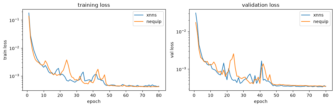
training time: xnn 759s nequip 733s
5. Evaluate both trained models on the held-out test set#
Identical evaluation for each: predict energy + forces (autograd) on all 50 test configurations and compute per-atom energy and force errors.
def eval_xnn(model):
    model.eval(); Ep, Er, na, Fp, Fr = [], [], [], [], []
    for s, i in zip(test_structs, range(len(xnn_test))):
        out = model(xnn_test[i].to(DEVICE))
        Ep.append(float(out["energy"].detach())); Er.append(s["energy"]); na.append(len(s["atomic_numbers"]))
        Fp.append(out["forces"].detach().cpu().numpy()); Fr.append(s["forces"])
    return map(np.array, (Ep, Er, na)), np.concatenate(Fp), np.concatenate(Fr)

def eval_nequip(model):
    model.eval(); Ep, Er, na, Fp, Fr = [], [], [], [], []
    for s, d in zip(test_structs, nequip_test):
        b = next(iter(NequipDataLoader([d], batch_size=1))).to(DEVICE)
        out = model(AtomicData.to_AtomicDataDict(b))
        Ep.append(float(out["total_energy"].sum().detach())); Er.append(s["energy"]); na.append(len(s["atomic_numbers"]))
        Fp.append(out["forces"].detach().cpu().numpy()); Fr.append(s["forces"])
    return map(np.array, (Ep, Er, na)), np.concatenate(Fp), np.concatenate(Fr)

def metrics(EpErNa, Fp, Fr):
    Ep, Er, na = EpErNa
    e = (Ep - Er) / na * 1000.0; f = (Fp - Fr) * 1000.0
    return dict(e_rmse=np.sqrt((e**2).mean()), e_mae=np.abs(e).mean(),
                f_rmse=np.sqrt((f**2).mean()), f_mae=np.abs(f).mean(),
                Ep=Ep/na, Er=Er/na, Fp=Fp, Fr=Fr)

res_x = metrics(*eval_xnn(trainer.model))
res_n = metrics(*eval_nequip(nequip_model))

print(f"{'metric':<22}{'xnn':>12}{'original NequIP':>18}")
print("-" * 52)
print(f"{'energy RMSE [meV/atom]':<22}{res_x['e_rmse']:>12.2f}{res_n['e_rmse']:>18.2f}")
print(f"{'energy MAE  [meV/atom]':<22}{res_x['e_mae']:>12.2f}{res_n['e_mae']:>18.2f}")
print(f"{'force  RMSE [meV/Å]':<22}{res_x['f_rmse']:>12.2f}{res_n['f_rmse']:>18.2f}")
print(f"{'force  MAE  [meV/Å]':<22}{res_x['f_mae']:>12.2f}{res_n['f_mae']:>18.2f}")
metric                        xnn   original NequIP
----------------------------------------------------
energy RMSE [meV/atom]       15.33             15.04
energy MAE  [meV/atom]       10.59             12.13
force  RMSE [meV/Å]           2.07              1.99
force  MAE  [meV/Å]           1.31              1.24
Side-by-side parity plots#
fig, ax = plt.subplots(2, 2, figsize=(9.5, 9))
rng = np.random.default_rng(0)
idx = rng.choice(res_x["Fr"].size, size=4000, replace=False)
for col, (res, name) in enumerate([(res_x, "xnn"), (res_n, "original NequIP")]):
    a0 = ax[0, col]
    lim = [min(res["Er"].min(), res["Ep"].min()), max(res["Er"].max(), res["Ep"].max())]
    a0.plot(lim, lim, "k--", lw=1); a0.scatter(res["Er"], res["Ep"], s=26, alpha=0.7)
    a0.set_xlabel("ref E/atom [eV]"); a0.set_ylabel("pred E/atom [eV]")
    a0.set_title(f"{name}: energy (RMSE {res['e_rmse']:.1f} meV/atom)")
    a1 = ax[1, col]
    fr, fp = res["Fr"].ravel()[idx], res["Fp"].ravel()[idx]
    lim = [min(fr.min(), fp.min()), max(fr.max(), fp.max())]
    a1.plot(lim, lim, "k--", lw=1); a1.scatter(fr, fp, s=6, alpha=0.3)
    a1.set_xlabel("ref force [eV/Å]"); a1.set_ylabel("pred force [eV/Å]")
    a1.set_title(f"{name}: forces (RMSE {res['f_rmse']:.1f} meV/Å)")
plt.tight_layout(); plt.savefig("argon_parity_xnn_vs_nequip.png", dpi=120); plt.show()
print("saved argon_parity_xnn_vs_nequip.png")
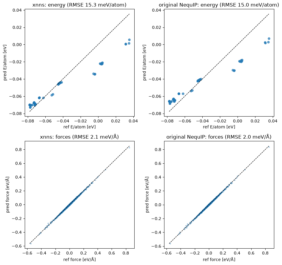
saved argon_parity_xnn_vs_nequip.png
6. xnn ASE calculator (deployment)#
xnn ships an ASE Calculator for the trained model, the same one used for the
xnn MACE, because every xnn model shares the AtomicGraph -> energy contract.
from ase import Atoms
from xnn.common.deploy import XNNCalculator

s = test_structs[0]
atoms = Atoms(numbers=s["atomic_numbers"], positions=s["pos"], cell=s["cell"], pbc=True)
atoms.calc = XNNCalculator(trainer.model.to("cpu"), cutoff=CUTOFF)
print(f"ASE single point: E = {atoms.get_potential_energy():.4f} eV "
      f"({atoms.get_potential_energy()/len(atoms)*1000:.1f} meV/atom) | "
      f"max|F| = {np.abs(atoms.get_forces()).max():.4f} eV/Å")
print(f"reference       : E = {s['energy']:.4f} eV")
ASE single point: E = -27.9015 eV (-69.8 meV/atom) | max|F| = 0.0871 eV/Å
reference       : E = -31.0395 eV
Summary: every stage compared#
stage |
result |
|---|---|
Data → graphs |
xnn and |
Model build |
identical architecture; parameter counts match except xnn’s 200-entry |
Same function? |
transplanting weights gives identical E and F on periodic Argon (float32 round-off; ~1e-15 in float64) |
Training |
same data / loss / optimiser / schedule → comparable loss curves and final losses |
Test accuracy |
energy and force RMSE/MAE agree between the two implementations |
The xnn NequIP is a faithful, dependency-light (only e3nn) re-implementation
of the original NequIP: it not only matches block-by-block (notebook 01) but
delivers an equivalent end-to-end training/testing pipeline on realistic Argon
data. The small residual differences in trained metrics come only from independent
random initialisation and data shuffling; apply the transplant of Section 3b
before training to start both from identical weights if exact-match training
curves are desired.
REF_stress is also present in the data; periodic stress training can be enabled
with compute_stress=True / non-zero stress_weight (autograd strain trick on the
xnn side, StressForceOutput upstream). The companion notebook
nequip_argon_density_md.ipynb uses exactly that to run NPT molecular dynamics
with both codes.