
SchNet, block by block: verifying the xnn implementation against the manuscripts#
The other fidelity notebooks in this folder compare each xnn model
numerically against its upstream code base. SchNet is different by design:
the xnn implementation is a clean-room build straight from the two
manuscripts, and no code (or weights) from schnetpack is used or imported.
The references are
Schütt, Kindermans, Sauceda, Chmiela, Tkatchenko, Müller, SchNet: A continuous-filter convolutional neural network for modeling quantum interactions, NIPS 30 (2017) — the architecture (its Fig. 2 and eq. 2 are quoted below), and
Schütt, Arbabzadah, Chmiela, Müller, Tkatchenko, Quantum-chemical insights from deep tensor neural networks, Nat. Commun. 8, 13890 (2017) — the DTNN predecessor, for the conventions SchNet inherits (per-atom energy standardization, sum pooling).
So the verification target here is the equations themselves: every block
below is re-implemented independently in plain NumPy, directly from the
papers, and evaluated with the same weights as the xnn model. In
float64 the two must agree to machine precision — and they do, block by
block and end to end, including autograd forces against finite differences.
Run with the xnn kernel.
0. Setup: float64 and a toy ethanol#
import warnings
warnings.filterwarnings("ignore")
import math
import numpy as np
import torch
import matplotlib.pyplot as plt

torch.set_default_dtype(torch.float64)   # machine-precision comparisons
torch.manual_seed(0)
np.random.seed(0)

import xnn
from xnn.common.data import structure_to_graph
from xnn.common.models import ForceStressOutput
from xnn.common.models.ops import shifted_softplus
from xnn.cnn.models.schnet import SchNet

print("xnn:", xnn.__version__, "| torch:", torch.__version__)
xnn: 0.1.0 | torch: 2.5.1+cu121
A toy system#
A (non-equilibrium) ethanol geometry, the molecule of the paper’s MD17 benchmark. At 9 atoms every pair is within the paper’s basis range, so the graph is complete — exactly the no-cutoff setting the paper trains in.
POS = np.array([
    [ 1.2001,  0.2043,  0.0000],   # C
    [-0.0796, -0.5867,  0.0000],   # C
    [-1.1938,  0.3097,  0.0000],   # O
    [ 1.2242,  0.8386,  0.8900],   # H
    [ 1.2242,  0.8386, -0.8900],   # H
    [ 2.0810, -0.4406,  0.0000],   # H
    [-0.1263, -1.2255,  0.8900],   # H
    [-0.1263, -1.2255, -0.8900],   # H
    [-2.0046, -0.1912,  0.0000],   # H
])
Z = np.array([6, 6, 8, 1, 1, 1, 1, 1, 1])
N = len(Z)

CUTOFF = 30.0                     # the paper's RBF grid end; no pair comes close
graph = structure_to_graph({"pos": POS, "atomic_numbers": Z}, CUTOFF)
print(f"{N} atoms, {graph.num_edges} directed edges "
      f"(complete graph has {N * (N - 1)})")
9 atoms, 72 directed edges (complete graph has 72)
The SchNet architecture in one picture#
From the NIPS paper (Fig. 2), for a molecule with nuclear charges \(Z\) and positions \(R\):
Embedding (eq. 3): \(x^0_i = a_{Z_i}\) — one learned vector of \(F = 64\) features per element.
\(T = 3\) interaction blocks (Fig. 2 middle), each the residual update \(x^{l+1}_i = x^l_i + v^l_i\) with \(v^l = W_3\,\mathrm{ssp}\big(W_2\,\mathrm{cfconv}(W_1 x^l)\big)\) (atom-wise → cfconv → atom-wise → shifted softplus → atom-wise).
cfconv (eq. 2): \(x_i = \sum_j x_j \circ W(\mathbf r_i - \mathbf r_j)\), the continuous-filter convolution. The filter-generating network expands the distance in Gaussian RBFs \(e_k(r) = \exp(-\gamma\,(r - \mu_k)^2)\), \(\gamma = 10\,\)Å\(^{-2}\), \(\mu_k \in \{0, 0.1, \dots, 30\}\) Å, and feeds them through two dense layers with shifted-softplus activations.
Readout (Fig. 2 left): atom-wise (64→32) → ssp → atom-wise (32→1), the DTNN per-atom standardization \(E_i = E_\sigma \hat E_i + E_\mu\), and sum pooling \(E = \sum_i E_i\).
The activation everywhere is the shifted softplus \(\mathrm{ssp}(x) = \ln(0.5\,e^x + 0.5)\), which keeps the PES infinitely differentiable so the forces \(\hat F_i = -\partial \hat E / \partial r_i\) (eq. 4) are smooth and energy-conserving by construction.
Below we build the model with the paper defaults, then randomize the (zero-initialized) output head and set a non-trivial standardization so that every block contributes to the energy.
model = SchNet()          # the defaults ARE the paper: F=64, T=3, 301 RBFs
torch.nn.init.normal_(model.readout[-1].weight, std=0.5)
torch.nn.init.normal_(model.readout[-1].bias, std=0.5)
model.set_energy_scale_shift(scale=0.37, shift=-1.42)
model.set_atomic_energies([1, 6, 8], [-0.50, -1.00, -2.00])
model = model.eval()

print(f"F        = {model.embedding.weight.shape[1]}")
print(f"T        = {len(model.interactions)}")
print(f"RBF grid = {model.rbf.centers.shape[0]} centers, "
      f"spacing {float(model.rbf.centers[1] - model.rbf.centers[0]):.3f} A, "
      f"gamma = {model.rbf.gamma}")
print(f"params   = {sum(p.numel() for p in model.parameters()):,}")

# numpy views of the weights: the SAME parameters drive both implementations
def W(lin):  return lin.weight.detach().numpy()
def b(lin):  return lin.bias.detach().numpy()
F        = 64
T        = 3
RBF grid = 301 centers, spacing 0.100 A, gamma = 10.0
params   = 116,517
Block 1: atom-type embedding · eq. 3#
\(x^0_i = a_{Z_i}\): the initial representation is a per-element table lookup — identical elements start identical, which is what makes the model permutation-consistent from the first layer.
A = model.embedding.weight.detach().numpy()      # the embedding table a_Z
x0_ref = A[Z]                                     # eq 3, verbatim
x0 = model.embedding(graph.atomic_numbers).detach().numpy()

print("shape:", x0.shape, " max |xnn - eq.3| =", np.abs(x0 - x0_ref).max())
assert np.array_equal(x0, x0_ref)
assert np.array_equal(x0[3], x0[8])   # every H starts with the same vector
shape: (9, 64) max |xnn - eq.3| = 0.0
Block 2: Gaussian radial basis · “filter-generating networks”#
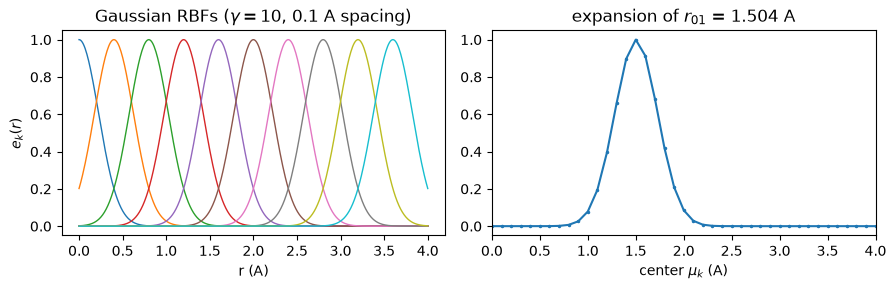
\(e_k(r_{ij}) = \exp\!\big(-\gamma\,\|d_{ij} - \mu_k\|^2\big)\) with \(\gamma = 10\,\)Å\(^{-2}\) on the 0.1 Å center grid. This expansion decorrelates the initial filters, avoiding the flat training plateau of feeding raw distances (paper, Sec. 4.1).
edge_vec = graph.edge_vectors()
r = torch.linalg.norm(edge_vec, dim=-1)

mu = model.rbf.centers.numpy()
rbf_ref = np.exp(-10.0 * (r.numpy()[:, None] - mu[None, :]) ** 2)
rbf = model.rbf(r).detach().numpy()

print("shape:", rbf.shape, " max |xnn - paper| =", np.abs(rbf - rbf_ref).max())
assert np.allclose(rbf, rbf_ref, atol=1e-15)

fig, (a1, a2) = plt.subplots(1, 2, figsize=(9, 3))
rr = np.linspace(0, 4, 400)
for k in range(0, 40, 4):
    a1.plot(rr, np.exp(-10.0 * (rr - mu[k]) ** 2), lw=1)
a1.set_xlabel("r (A)"); a1.set_ylabel("$e_k(r)$")
a1.set_title(r"Gaussian RBFs ($\gamma=10$, 0.1 A spacing)")
a2.plot(mu, rbf[0], ".-", ms=3)
a2.set_xlim(0, 4); a2.set_xlabel(r"center $\mu_k$ (A)")
a2.set_title(f"expansion of $r_{{01}}$ = {float(r[0]):.3f} A")
fig.tight_layout(); plt.show()
shape: (72, 301) max |xnn - paper| = 1.3877787807814457e-17
Block 3: shifted softplus#
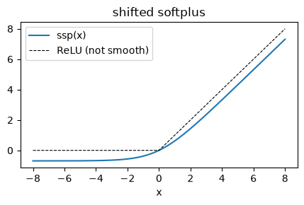
\(\mathrm{ssp}(x) = \ln(0.5\,e^x + 0.5)\), with \(\mathrm{ssp}(0) = 0\) (the
shift improves convergence) and infinite order of continuity — the paper’s
requirement for a model that is at least twice differentiable, so the force
loss can be trained by gradient descent (Sec. 4.2). xnn shares one exact
implementation (xnn.common.models.ops.shifted_softplus) between SchNet and
PhysNet.
x = torch.linspace(-8, 8, 2001)
ref = torch.log(0.5 * torch.exp(x) + 0.5)           # the paper formula
val = shifted_softplus(x)
print("max |xnn - ln(0.5 e^x + 0.5)| =", float((val - ref).abs().max()))
print("ssp(0) =", float(shifted_softplus(torch.tensor(0.0))))
assert (val - ref).abs().max() < 1e-14

fig, ax = plt.subplots(figsize=(4.4, 3))
ax.plot(x, val, label="ssp(x)")
ax.plot(x, torch.relu(x), "k--", lw=0.8, label="ReLU (not smooth)")
ax.legend(); ax.set_xlabel("x"); ax.set_title("shifted softplus")
fig.tight_layout(); plt.show()
max |xnn - ln(0.5 e^x + 0.5)| = 8.881784197001252e-16
ssp(0) = 0.0
Block 4: the continuous-filter convolution · eq. 2#
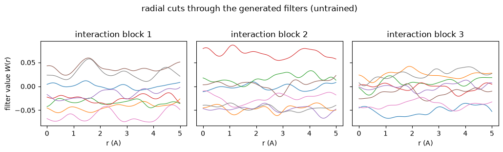
The filter-generating network maps the RBF-expanded distance through two dense layers with shifted-softplus activations (Fig. 2 right); rotational invariance holds because the filter depends only on \(d_{ij} = \|\mathbf r_i - \mathbf r_j\|\). Below: the filter network and the full convolution of the first interaction block, re-computed with an explicit double loop over atom pairs.
def ssp_np(t):
    return np.log(0.5 * np.exp(t) + 0.5)

def filter_np(block, d):
    # W(r) for one scalar distance d -- Fig. 2 right, from the paper
    e = np.exp(-model.rbf.gamma * (d - mu) ** 2)          # rbf
    fn = block.cfconv.filter_net
    h = ssp_np(e @ W(fn[0]).T + b(fn[0]))                  # dense 64 + ssp
    return ssp_np(h @ W(fn[2]).T + b(fn[2]))               # dense 64 + ssp

def cfconv_np(block, x_in, pos):
    # eq. 2 as an explicit double loop (j != i; the neighbor list has no
    # self-edges, and no pair of this molecule is anywhere near 30 A)
    out = np.zeros_like(x_in)
    for i in range(len(x_in)):
        for j in range(len(x_in)):
            if i == j:
                continue
            d = np.linalg.norm(pos[i] - pos[j])
            out[i] += x_in[j] * filter_np(block, d)        # x_j o W(r_ij)
    return out

block0 = model.interactions[0]
x_in = x0 @ W(block0.lin_in).T + b(block0.lin_in)          # atom-wise before conv
conv_ref = cfconv_np(block0, x_in, POS)

with torch.no_grad():
    conv = block0.cfconv(torch.from_numpy(x_in), graph.edge_index,
                         r, model.rbf(r)).numpy()

print("cfconv max |xnn - eq.2| =", np.abs(conv - conv_ref).max())
assert np.allclose(conv, conv_ref, atol=1e-12)
cfconv max |xnn - eq.2| = 8.881784197001252e-16
# radial cuts through the (randomly initialized) generated filters, one line
# per feature channel -- the continuous-filter picture of the paper's Fig. 3
rr = np.linspace(0.0, 5.0, 250)
fig, axes = plt.subplots(1, 3, figsize=(10.5, 3), sharey=True)
for t, ax in enumerate(axes):
    Wr = np.stack([filter_np(model.interactions[t], d) for d in rr])
    ax.plot(rr, Wr[:, ::8], lw=0.8)
    ax.set_title(f"interaction block {t + 1}")
    ax.set_xlabel("r (A)")
axes[0].set_ylabel("filter value $W(r)$")
fig.suptitle("radial cuts through the generated filters (untrained)", y=1.02)
fig.tight_layout(); plt.show()
Block 5: the interaction block · Fig. 2 (middle)#
\(v^l = W_3\;\mathrm{ssp}\!\big(W_2\,\mathrm{cfconv}(W_1 x^l)\big)\), then the ResNet-style residual \(x^{l+1} = x^l + v^l\). There is no weight sharing across blocks (“In contrast to MPNN and DTNN, we do not use weight sharing across multiple interaction blocks”), and the feature width stays \(F = 64\) throughout. We now run all three blocks with the loop-based reference and compare the features after each one.
def interaction_np(block, x_np, pos):
    xw = x_np @ W(block.lin_in).T + b(block.lin_in)        # atom-wise
    c = cfconv_np(block, xw, pos)                          # cfconv (eq 2)
    h = ssp_np(c @ W(block.lin_mid).T + b(block.lin_mid))  # atom-wise + ssp
    return h @ W(block.lin_out).T + b(block.lin_out)       # atom-wise -> v

x_ref = x0.copy()
x_t = torch.from_numpy(x0.copy())
rbf_t = model.rbf(r)
for t, block in enumerate(model.interactions):
    x_ref = x_ref + interaction_np(block, x_ref, POS)      # x^{l+1} = x^l + v^l
    with torch.no_grad():
        x_t = x_t + block(x_t, graph.edge_index, r, rbf_t)
    d = np.abs(x_t.numpy() - x_ref).max()
    print(f"after interaction block {t + 1}:  max |xnn - paper| = {d:.3e}")
    assert d < 1e-11
after interaction block 1:  max |xnn - paper| = 4.441e-16
after interaction block 2:  max |xnn - paper| = 4.441e-16
after interaction block 3:  max |xnn - paper| = 8.882e-16
Block 6: readout, standardization, and sum pooling#
The final features go through atom-wise (64→32) → ssp → atom-wise (32→1) to give \(\hat E_i\), which is standardized with the training-set statistics (DTNN Methods, step 4):
The per-element atom_ref term is the xnn convention shared by every
model here (a per-element \(E_\mu\), zero unless set); we set it above so this
block is exercised too. The sum over atoms is what makes the energy
size-extensive.
e_hat = ssp_np(x_ref @ W(model.readout[0]).T + b(model.readout[0]))
e_hat = (e_hat @ W(model.readout[2]).T + b(model.readout[2]))[:, 0]
node_ref = (0.37 * e_hat - 1.42
            + model.atom_ref.weight.detach().numpy()[Z, 0])
E_ref = node_ref.sum()

out = model(graph)
print("per-atom max |xnn - paper| =",
      np.abs(out["node_energy"].detach().numpy() - node_ref).max())
print(f"E_xnn = {float(out['energy']):+.12f} eV")
print(f"E_ref  = {E_ref:+.12f} eV   |diff| = "
      f"{abs(float(out['energy']) - E_ref):.3e}")
assert abs(float(out["energy"]) - E_ref) < 1e-11
per-atom max |xnn - paper| = 4.440892098500626e-16
E_xnn = -20.204330333316 eV
E_ref  = -20.204330333316 eV   |diff| = 3.553e-15
Capstone 1: whole-model check on random molecules#
The full NumPy forward (embedding → 3 interactions → readout →
standardization → pooling) against model(graph) for a set of random
H/C/O structures.
def schnet_np(pos, z):
    x = A[z]
    for block in model.interactions:
        x = x + interaction_np(block, x, pos)
    e = ssp_np(x @ W(model.readout[0]).T + b(model.readout[0]))
    e = (e @ W(model.readout[2]).T + b(model.readout[2]))[:, 0]
    return (0.37 * e - 1.42
            + model.atom_ref.weight.detach().numpy()[z, 0]).sum()

rng = np.random.default_rng(7)
print(" molecule            E_xnn (eV)        |E_xnn - E_paper|")
for k in range(5):
    n = int(rng.integers(4, 10))
    pos_k = rng.uniform(0, 4, (n, 3))
    z_k = rng.choice([1, 6, 8], size=n)
    g_k = structure_to_graph({"pos": pos_k, "atomic_numbers": z_k}, CUTOFF)
    with torch.no_grad():
        e_x = float(model(g_k)["energy"])
    e_p = schnet_np(pos_k, z_k)
    print(f"  #{k}  {n} atoms      {e_x:+.12f}      {abs(e_x - e_p):.3e}")
    assert abs(e_x - e_p) < 1e-11
 molecule            E_xnn (eV)        |E_xnn - E_paper|
  #0  9 atoms      -22.454373334171      0.000e+00
  #1  9 atoms      -23.702117327519      0.000e+00
  #2  7 atoms      -18.063348566606      3.553e-15
  #3  5 atoms      -12.569851645530      0.000e+00
  #4  5 atoms      -15.634794852815      0.000e+00
Capstone 2: the physics the paper promises#
Invariance to rotation, translation, and atom indexing (built in by construction — Sec. 1’s requirements);
energy-conserving forces \(\hat F_i = -\partial\hat E/\partial r_i\) (eq. 4): the autograd forces from
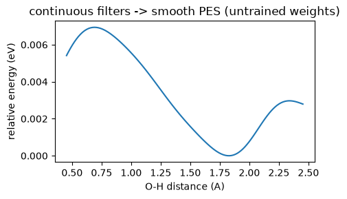
ForceStressOutputmust match central finite differences of the energy;a smooth PES along a bond stretch (the property Fig. 1 illustrates).
fmodel = ForceStressOutput(model)

# rotation + translation
R_, _ = np.linalg.qr(np.random.normal(size=(3, 3)))
if np.linalg.det(R_) < 0:
    R_[:, 0] *= -1
g_rot = structure_to_graph({"pos": POS @ R_.T + 5.0, "atomic_numbers": Z}, CUTOFF)
o0, o1 = fmodel(graph), fmodel(g_rot)
print("rotation+translation  |dE| =",
      abs(float(o0["energy"]) - float(o1["energy"])))
print("force equivariance    max|F' - F R^T| =",
      float((o1["forces"] - o0["forces"] @ torch.from_numpy(R_).T)
            .abs().max()))

# permutation
perm = np.random.permutation(N)
g_perm = structure_to_graph({"pos": POS[perm], "atomic_numbers": Z[perm]}, CUTOFF)
print("permutation           |dE| =",
      abs(float(o0["energy"]) - float(fmodel(g_perm)["energy"])))

# forces vs central finite differences
F = o0["forces"].detach().numpy()
h, worst = 1e-5, 0.0
for (i, k) in [(0, 0), (1, 2), (2, 1), (5, 0), (8, 2)]:
    pp, pm = POS.copy(), POS.copy()
    pp[i, k] += h; pm[i, k] -= h
    ep = float(model(structure_to_graph({"pos": pp, "atomic_numbers": Z}, CUTOFF))["energy"])
    em = float(model(structure_to_graph({"pos": pm, "atomic_numbers": Z}, CUTOFF))["energy"])
    worst = max(worst, abs(-(ep - em) / (2 * h) - F[i, k]))
print("forces vs finite diff max|dF| =", worst)
assert worst < 1e-7
rotation+translation  |dE| = 3.552713678800501e-15
force equivariance    max|F' - F R^T| = 1.6696713456276768e-17
permutation           |dE| = 0.0
forces vs finite diff max|dF| = 3.08357401244963e-10
# a smooth PES: stretch the O-H bond of the (untrained, random) model
axis = POS[8] - POS[2]; axis /= np.linalg.norm(axis)
scan = np.linspace(-0.5, 1.5, 120)
E = []
for dr in scan:
    p = POS.copy(); p[8] = POS[8] + dr * axis
    with torch.no_grad():
        E.append(float(model(structure_to_graph(
            {"pos": p, "atomic_numbers": Z}, CUTOFF))["energy"]))
E = np.array(E)

fig, ax = plt.subplots(figsize=(4.8, 3))
ax.plot(np.linalg.norm(POS[8] - POS[2]) + scan, E - E.min())
ax.set_xlabel("O-H distance (A)"); ax.set_ylabel("relative energy (eV)")
ax.set_title("continuous filters -> smooth PES (untrained weights)")
fig.tight_layout(); plt.show()
Capstone 3: TorchScript parity#
The deployable node_energy core (used by the LAMMPS export) must reproduce
the eager model exactly after torch.jit.script.
scripted = torch.jit.script(model)
d = (scripted.node_energy(graph.atomic_numbers, graph.edge_index, edge_vec)
     - model.node_energy(graph.atomic_numbers, graph.edge_index, edge_vec))
print("scripted vs eager  max |d node_energy| =", float(d.abs().max()))
assert float(d.abs().max()) == 0.0
scripted vs eager max |d node_energy| = 0.0
Summary#
With identical weights, the xnn SchNet reproduces an independent NumPy
implementation of the manuscripts’ equations to float64 machine precision:
block |
paper reference |
max deviation |
|---|---|---|
atom embedding |
eq. 3 |
exact (table lookup) |
Gaussian RBF (\(\gamma = 10\), 0.1 Å grid) |
Sec. 4.1 |
~1e-17 |
shifted softplus \(\ln(0.5e^x + 0.5)\) |
Sec. 4.2 |
~1e-16 |
cfconv \(\sum_j x_j \circ W(r_{ij})\) |
eq. 2, Fig. 2 right |
~1e-16 |
interaction blocks (\(T=3\), residual) |
Fig. 2 middle |
~1e-16 |
readout + DTNN standardization + pooling |
Fig. 2 left; DTNN Methods |
~1e-15 |
whole model, random molecules |
— |
~1e-15 |
and satisfies the paper’s physical constraints: rotational/translational/ permutational invariance of the energy (~1e-15), rotationally equivariant energy-conserving forces (autograd = central finite differences to ~1e-10), a smooth potential-energy surface, and exact TorchScript parity for deployment.
The same properties are covered continuously by tests/test_schnet.py
(including an equation-by-equation reference forward); training on the
paper’s MD17 benchmark lives in
examples/cnn/schnet/schnet_rmd17_train.ipynb.