Training ReaxFF-nn on rMD17 (malonaldehyde)

ReaxFF (van Duin et al., J. Phys. Chem. A 105, 9396, 2001) is the bond-order reactive force field: every valence term is written in terms of distance-derived bond orders, so bonds can break and form smoothly, and partial charges are re-equilibrated at every geometry (EEM). ReaxFF-nn (Guo et al., Comput. Mater. Sci. 172, 109393, 2020; Xue et al., PCCP 23, 19457, 2021) replaces the closed-form bond-order correction (and, optionally, the bond energy) with small per-species / per-bond neural networks — turning the force field into a machine-learning potential whose every parameter is trainable by gradient descent, while keeping the physically-motivated ReaxFF functional form for everything else (angles, torsions, EEM electrostatics, van der Waals, hydrogen bonds).

This notebook does what the ffnn family exists for: it trains a force field. Starting from a generic, untrained seed library (xnn.ffnn.models.template_library — plausible radii, valences and EEM values, randomly initialized networks), it fits energies and forces of the rMD17 malonaldehyde trajectory (PBE/def2-SVP). The sampled conformer is the dialdehyde form, O=CH–CH₂–CH=O — a small conjugated molecule whose chemically distinct bonds (C=O double bonds, C–C single bonds, aldehyde and methylene C–H) are exactly what a bond-order force field has to resolve. Two kinds of parameters are trained at once:

• the message-passing bond-order network fm (the ReaxFF-nn core, one small all-sigmoid network per element), with the bond energy kept in its classical Morse-like form (EnergyFunction = 0) so that the dissociation limit stays tied to the physical Desi parameters — the fully-neural bond energy (EnergyFunction = 1) is available via template_library(..., energy_function=1);

• a set of classical parameter groups (bond dissociation energies, valence-angle and torsion prefactors, …) refit by backprop — the other headline of this family. Exponent-type parameters (bond-order decay rates, the V2 torsion envelope, vdW steepness) are deliberately kept frozen: they control the asymptotics of the force field, which equilibrium-only training data cannot constrain.

The trained model is exported back to a portable ffield.json library, which the companion notebook reaxff_md_bond_orders.ipynb uses for molecular dynamics, bond-order and charge analysis, and a bond-dissociation study. Both notebooks also compare against the original classical ReaxFF with published parameters — the same ReaxFF class runs a standard ffield text file directly, networks and training entirely optional.

0. Setup and data

import io, os, re, time, warnings
warnings.filterwarnings("ignore")
import contextlib

import numpy as np
import torch
import matplotlib.pyplot as plt

torch.manual_seed(0)
rng = np.random.default_rng(0)

from xnn.common.data import load_dataset, AtomicDataset, collate

# rMD17 malonaldehyde: C3H4O2, 9 atoms, 100k configurations sampled at 500 K,
# recomputed at PBE/def2-SVP. A modest subsample keeps this notebook to a few
# minutes of CPU time.
structures = load_dataset("rmd17", molecule="malonaldehyde", split="train")
idx = rng.permutation(len(structures))[:800]
subset = [structures[i] for i in idx]
n_train, n_val = 640, 80

energies = np.array([s["energy"] for s in subset])
print(f"{len(subset)} structures of {len(subset[0]['atomic_numbers'])} atoms; "
      f"energy spread {1000 * energies.std():.0f} meV (std), "
      f"range {1000 * np.ptp(energies):.0f} meV")

800 structures of 9 atoms; energy spread 189 meV (std), range 1338 meV

1. The seed force field

template_library builds a complete-but-untrained ReaxFF-nn parameter library. Its bond-order exponentials are anchored so that BO(rₑ) ≈ 0.85 at the covalent bond length and BO ≈ 10⁻⁴ at the neighbor-list cutoff — bond orders (and with them every valence term) then vanish smoothly at the list boundaries, which is what keeps molecular dynamics conservative. It is a starting point, not a validated force field. The only calibration done by hand is the per-element reference energies (atomic), initialized so the seed model’s mean energy matches the data (rMD17 stores absolute DFT energies); they stay trainable so the optimizer can refine the offset.

from xnn.ffnn.models import template_library, ReaxFF

lib = template_library(["C", "H", "O"], nn=True, seed=0, energy_function=0)
seed_model = ReaxFF(lib, trainable=("atomic",))

calib = collate([AtomicDataset(subset[:32], cutoff=seed_model.cutoff)[i]
                 for i in range(32)])
with torch.no_grad():
    shift = (seed_model(calib)["energy"].mean() - calib.energy.mean()) / 9
    seed_model.params["atomic"] += shift

os.makedirs("runs/reaxff_rmd17", exist_ok=True)
seed_path = "runs/reaxff_rmd17/ffield_seed.json"
seed_model.export_library().save(seed_path)
print(f"seed library written to {seed_path} "
      f"(atomic-energy shift {float(shift):+.1f} eV/atom)")

seed library written to runs/reaxff_rmd17/ffield_seed.json (atomic-energy shift +806.4 eV/atom)

2. Train through the standard xnn pipeline

The model registers as "reaxff", so the usual config → Trainer route applies. trainable lists the classical parameter groups the optimizer may refit alongside the (always-trainable) ReaxFF-nn networks. The loss is the standard per-atom energy + force objective; forces differentiate the whole functional form (EEM solve included), which is what makes classical-parameter refitting by backprop work.

from xnn.common.config import from_dict
from xnn.common.train import Trainer

cfg = from_dict({
    "model": {
        "name": "reaxff",
        "cutoff": 10.0,                      # nonbonded/EEM cutoff (standard)
        "ffield": seed_path,
        "trainable": ["atomic", "Desi", "Depi", "Depp", "ovun1",
                      "ang_val1", "ang_val2", "ang_theta0",
                      "tor_V1", "tor_V2", "tor_V3"],
    },
    "data": {"cutoff": 10.0, "batch_size": 16},
    "optim": {"lr": 5e-3, "epochs": 300, "energy_weight": 1.0,
              "force_weight": 0.3, "scheduler": "cosine"},
    "device": "cpu",
    "output_dir": "runs/reaxff_rmd17",
})

train_set = AtomicDataset(subset[:n_train], cutoff=cfg.model.cutoff)
val_set = AtomicDataset(subset[n_train:n_train + n_val],
                        cutoff=cfg.model.cutoff)
test_set = AtomicDataset(subset[n_train + n_val:], cutoff=cfg.model.cutoff)

trainer = Trainer(cfg, train_set, val_set, test_set)
t0 = time.time()
log = io.StringIO()
with contextlib.redirect_stdout(log):
    history = trainer.fit()
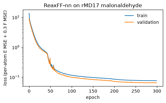
print(f"trained {cfg.optim.epochs} epochs in {time.time() - t0:.0f} s")
print("final:", {k: {m: round(float(x), 5) for m, x in v.items()}
                 for k, v in history.items()})

trained 300 epochs in 563 s
final: {'train': {'energy_mse': 0.00014, 'force_mse': 0.25271, 'loss': 0.07595}, 'val': {'energy_mse': 0.0001, 'force_mse': 0.21473, 'loss': 0.06452}, 'test': {'energy_mse': 0.00013, 'force_mse': 0.21937, 'loss': 0.06594}}

# learning curve, parsed from the trainer's per-epoch log
epochs, tr_loss, va_loss = [], [], []
for line in log.getvalue().splitlines():
    m = re.match(r"epoch\s+(\d+) \| train loss ([\d.e+-]+|nan)"
                 r" \| val loss ([\d.e+-]+|nan)", line)
    if m:
        epochs.append(int(m.group(1)))
        tr_loss.append(float(m.group(2)))
        va_loss.append(float(m.group(3)))

fig, ax = plt.subplots(figsize=(5.4, 3.4))
ax.semilogy(epochs, tr_loss, label="train")
ax.semilogy(epochs, va_loss, label="validation")
ax.set_xlabel("epoch")
ax.set_ylabel("loss (per-atom E MSE + 0.3 F MSE)")
ax.set_title("ReaxFF-nn on rMD17 malonaldehyde")
ax.legend(frameon=False)
fig.tight_layout()
fig.savefig("reaxff_loss_curves.png", dpi=150)
plt.show()

3. Test-set accuracy: original vs seed vs trained

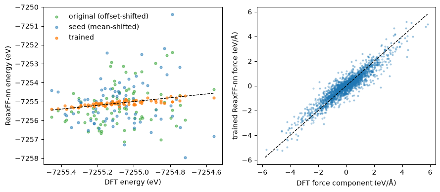
Energy and force parity on held-out configurations. Besides the seed and the trained libraries, the same test set is evaluated with the original classical ReaxFF: the published C/H/O combustion parameterization of Chenoweth, van Duin and Goddard (J. Phys. Chem. A 112, 1040, 2008), read directly from the SEAMM .frc force-field format (CHO_cho_2008 (shipped with xnn in the SEAMM .frc format), shipped alongside this notebook). Nothing about it is fitted to this data — it uses its own absolute energy reference, so a constant offset (fitted on the training split) is removed before comparing energies. It anchors the comparison: transferable published parameters cover all of C/H/O combustion chemistry at once, but malonaldehyde’s conjugated dialdehyde backbone is far from that parameterization target, and both metrics show it.

A classical functional form with a small message network will not reach the meV accuracy of large descriptor/GNN models on this benchmark — the point of a learnable force field is different: a physically interpretable, reactive, portable parameterization (every fitted number is still a ReaxFF parameter) whose accuracy improves systematically as more parameter groups, data and epochs are allowed. Note also what the fit cannot know: the training data samples thermal (≤ 500 K) configurations only, so regions far off that manifold — stretched bonds, close contacts — inherit the seed’s generic parameters rather than data (the companion notebook makes this concrete, including where the original field in turn beats the trained one).

from xnn.common.models import ForceStressOutput

model = trainer.module.model          # the trained ReaxFF inside the wrapper
fs = trainer.module
model.eval()


def collect(wrapped):
    es, fs_ = [], []
    for i in range(len(test_set)):
        out = wrapped(test_set[i])
        es.append(float(out["energy"][0]))
        fs_.append(out["forces"].detach().numpy())
    return np.array(es), np.concatenate([f.ravel() for f in fs_])


seed_model2 = ReaxFF(seed_path)           # untouched seed, for comparison
e_seed, f_seed = collect(ForceStressOutput(seed_model2))
e_pred, f_pred = collect(fs)
e_ref = np.array([float(test_set[i].energy[0]) for i in range(len(test_set))])
f_ref = np.concatenate([test_set[i].forces.numpy().ravel()
                        for i in range(len(test_set))])

# the original published field, read from the standard ffield text format;
# its constant energy reference is fitted on (a sample of) the training split
orig_model = ForceStressOutput(ReaxFF("CHO_cho_2008"))
off = np.mean([float(orig_model(train_set[i])["energy"][0])
               - float(train_set[i].energy[0]) for i in range(0, n_train, 10)])
e_orig, f_orig = collect(orig_model)
e_orig -= off

for name, e, f in (("original", e_orig, f_orig), ("seed", e_seed, f_seed),
                   ("trained", e_pred, f_pred)):
    print(f"{name:8s} E MAE {1000 * np.abs(e - e_ref).mean():8.1f} meV | "
          f"F MAE {np.abs(f - f_ref).mean():6.3f} eV/A")

fig, axes = plt.subplots(1, 2, figsize=(9, 4))
lo, hi = e_ref.min(), e_ref.max()
axes[0].plot([lo, hi], [lo, hi], "k--", lw=1)
axes[0].scatter(e_ref, e_orig, s=12, alpha=0.5, color="C2",
                label="original (offset-shifted)")
axes[0].scatter(e_ref, e_seed - e_seed.mean() + e_ref.mean(), s=12,
                alpha=0.5, label="seed (mean-shifted)")
axes[0].scatter(e_ref, e_pred, s=12, alpha=0.7, label="trained")
axes[0].set_xlabel("DFT energy (eV)")
axes[0].set_ylabel("ReaxFF-nn energy (eV)")
axes[0].legend(frameon=False)
lim = np.abs(f_ref).max()
axes[1].plot([-lim, lim], [-lim, lim], "k--", lw=1)
axes[1].scatter(f_ref, f_pred, s=4, alpha=0.3)
axes[1].set_xlabel("DFT force component (eV/Å)")
axes[1].set_ylabel("trained ReaxFF-nn force (eV/Å)")
fig.tight_layout()
fig.savefig("reaxff_parity.png", dpi=150)
plt.show()

original E MAE    811.4 meV | F MAE  5.917 eV/A
seed     E MAE    905.0 meV | F MAE  4.943 eV/A
trained  E MAE     82.7 meV | F MAE  0.350 eV/A

4. Export the trained force field

export_library() unpacks the trained tensors back into a flat parameter library (energies in kcal/mol, networks included) and save writes it in the ReaxFF-nn JSON format — a portable artifact: reload it here with ReaxFF("runs/reaxff_rmd17/ffield_trained.json"), or hand it to other ReaxFF-nn-aware codes. And because every fitted number is still a ReaxFF parameter, the result can be read: the refit sigma-bond dissociation energies below are the force field’s own statement of how strong it now thinks each bond is.

trained_path = "runs/reaxff_rmd17/ffield_trained.json"
model.export_library().save(trained_path)

# round-trip check: the reloaded library reproduces the trained model
# (to float32 round-off of the kcal/mol<->eV conversions; exact in float64)
reloaded = ReaxFF(trained_path)
g = test_set[0]
diff = abs(float(reloaded(g)["energy"][0]) - float(model(g)["energy"][0]))
print(f"saved {trained_path}; reload round-trip |dE| = {diff:.2e} eV")

lib_out = reloaded.export_library()
print("refit sigma-bond dissociation energies (seed value: 120 kcal/mol):")
for bd in ("C-O", "C-C", "C-H", "H-O"):
    key = f"Desi_{bd}" if f"Desi_{bd}" in lib_out.p else \
        f"Desi_{'-'.join(reversed(bd.split('-')))}"
    print(f"  {bd}: {lib_out.p[key]:7.1f} kcal/mol")

saved runs/reaxff_rmd17/ffield_trained.json; reload round-trip |dE| = 0.00e+00 eV
refit sigma-bond dissociation energies (seed value: 120 kcal/mol):
  C-O:   160.9 kcal/mol
  C-C:    48.5 kcal/mol
  C-H:   231.4 kcal/mol
  H-O:    91.3 kcal/mol