
DFT-D4 in xnn: reproducing examples of the D4 paper#
Caldeweyher, Ehlert, Hansen, Neugebauer, Spicher, Bannwarth & Grimme, J. Chem. Phys. 150, 154122 (2019)
introduce the D4 dispersion model: atomic dynamic polarizabilities that depend on the
atomic partial charge (eq 2, classical EEQ charges) and the coordination number
(eq 8), integrated to pairwise \(C_6\) coefficients (eq 9) and used in a BJ-damped
two-body plus ATM three-body dispersion energy (eqs 18–28). This notebook uses xnn’s
independent implementation (xnn.common.models.D4Dispersion, verified against the
reference dftd4 code to machine precision in examples/fidelity_checks/d4_verification.ipynb)
to reproduce, without any external quantum-chemistry data:
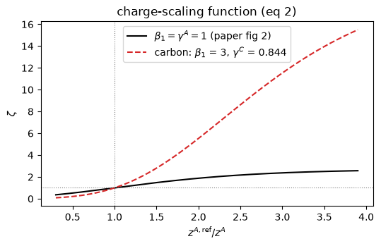
the charge-scaling function \(\zeta\) of fig 2;
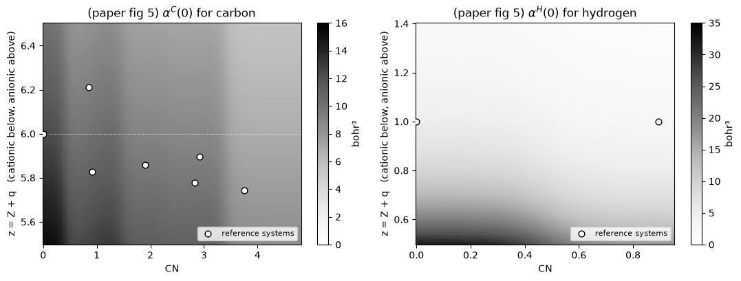
the charge- and CN-dependence of the static carbon and hydrogen polarizabilities of fig 5;
the atom-in-molecule polarizabilities and the molecular \(C_6\) of (3Z)-hexen-1-yne of fig 3(b) and the text of sec II (\(C_6^{\rm mol}\)(D4) = 1949.5, D3 = 1893.0, TD-DFT = 2103.1 \(E_h\,a_0^6\));
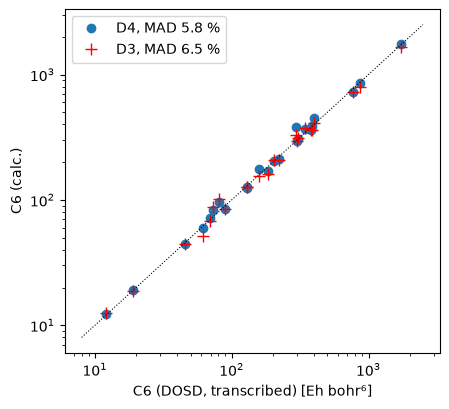
molecular \(C_6\) coefficients in the spirit of table III (the DOSD benchmark), D4 vs D3;
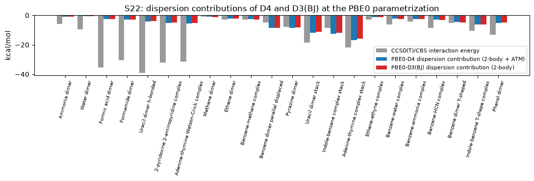
the charge dependence that D3 cannot express, and the D4 vs D3(BJ) dispersion contributions to the S22 interaction energies (sec III.B).
Everything runs with the PBE0-D4 parameters (s6 = 1, s8 = 1.20065498, a1 = 0.40085597, a2 = 5.02928789, s9 = 1, alp = 16), the paper’s default bj-eeq-atm variant.
import logging, warnings
logging.disable(logging.WARNING)
warnings.filterwarnings("ignore")

import numpy as np
import torch
import matplotlib.pyplot as plt
from ase import Atoms
from ase.build import molecule

torch.set_default_dtype(torch.float64)

import xnn
from xnn.common.data import structure_to_graph
from xnn.common.models import D4Dispersion, DFTD4, c6_matrix
from xnn.common.models import d3
from xnn.common.models.d4 import BOHR, HARTREE, PBE0_D4

d4 = D4Dispersion()          # PBE0-D4, bj-eeq-atm, upstream cutoffs
print("xnn", xnn.__version__, "| PBE0-D4:", PBE0_D4)

def run_d4(atoms, charge=0.0, model=d4):
    g = structure_to_graph({"pos": atoms.positions, "atomic_numbers": atoms.numbers, "total_charge": charge}, model.cutoff)
    out = model(g)
    out["c6"] = c6_matrix(out["dynamic_polarizabilities"])
    return {k: v.detach() for k, v in out.items()}

# PBE0-D3(BJ) (Grimme, Ehrlich & Goerigk 2011) through xnn's D3 tables, for the comparisons
D3_PBE0 = dict(s6=1.0, s8=1.2177, a1=0.4145, a2=4.8593)

def d3_pairs(atoms):
    z = torch.tensor(atoms.numbers); pos = torch.tensor(atoms.positions) / d3.d3_autoang
    n = len(z); ii, jj = torch.meshgrid(torch.arange(n), torch.arange(n), indexing="ij")
    off = ii != jj
    i, j = ii[off], jj[off]
    r = torch.linalg.norm(pos[i] - pos[j], dim=-1)
    cn = d3._ncoord(z[i], z[j], r, i, n)
    c6 = d3._getc6(z[ii.reshape(-1)], z[jj.reshape(-1)], cn[ii.reshape(-1)], cn[jj.reshape(-1)], d3.d3_c6ab).reshape(n, n)
    return z, r, i, j, c6

def run_d3(atoms):
    z, r, i, j, c6 = d3_pairs(atoms)
    e = float(d3.edisp(z, r, i, j, **D3_PBE0).sum()) if len(z) > 1 else 0.0   # hartree, two-body only
    return {"energy_au": e, "c6": c6}
xnn 0.2.1 | PBE0-D4: {'s6': 1.0, 's8': 1.20065498, 'a1': 0.40085597, 'a2': 5.02928789, 's9': 1.0, 'alp': 16.0}
1. The charge-scaling function ζ · fig 2, eq 2#
Fig 2 of the paper plots \(\zeta\) for \(\beta_1 = \gamma^A = 1\): no scaling when the atom carries its reference charge (the crossing at 1), enhanced polarizability for anions (\(z^{A,\rm ref}/z^A < 1\)) and suppressed for cations. The production model uses \(\beta_1 = 3\) and \(\gamma^A = 2\,\eta^A\) with the element’s chemical hardness; both curves are shown for carbon.
def zeta(a, c, ratio):
    return np.exp(a * (1 - np.exp(c * (1 - ratio))))

ratio = np.linspace(0.3, 3.9, 400)
eta_c = float(d4.d4.hardness[6])
plt.figure(figsize=(5.5, 3.6))
plt.plot(ratio, zeta(1.0, 1.0, ratio), "k", label=r"$\beta_1 = \gamma^A = 1$ (paper fig 2)")
plt.plot(ratio, zeta(d4.d4.ga, d4.d4.gc * eta_c, ratio), "C3--", label=rf"carbon: $\beta_1$ = {d4.d4.ga:.0f}, $\gamma^C$ = {d4.d4.gc * eta_c:.3f}")
plt.axhline(1, color="gray", ls=":", lw=0.8); plt.axvline(1, color="gray", ls=":", lw=0.8)
plt.xlabel(r"$z^{A,\mathrm{ref}} / z^A$"); plt.ylabel(r"$\zeta$"); plt.legend(); plt.title("charge-scaling function (eq 2)")
plt.tight_layout(); plt.show()
2. α(0) of carbon and hydrogen vs charge and coordination number · fig 5#
Fig 5 maps the static atom-in-molecule polarizability \(\alpha^A(0)\) (bohr³) over the
two model coordinates, the effective nuclear charge \(z = Z + q\) (cationic below,
anionic above \(Z\)) and the coordination number. The reference systems (white circles)
sit at their own \((\mathrm{CN}^{A,\rm ref}, z^{A,\rm ref})\) and are reproduced exactly at those
points; everywhere else the Gaussian weighting of eq 8 and the charge scaling of eq 2
interpolate. Both maps are generated directly from xnn’s DFTD4 building blocks.
core = d4.d4

def alpha_map(Z, cn_range, z_range, n=161):
    cn = torch.linspace(*cn_range, n); z = torch.linspace(*z_range, n)
    CN, ZZ = torch.meshgrid(cn, z, indexing="xy")
    zs = torch.full(CN.shape, Z, dtype=torch.long).reshape(-1)
    q = (ZZ - core.zeff[Z]).reshape(-1)          # partial charge behind z = Z_eff + q
    w = core.reference_weights(zs, CN.reshape(-1), q)
    alpha = core.dynamic_polarizabilities(zs, w)[:, 0].reshape(CN.shape)
    nref = int(core.nref[Z])
    refs = (core.refcn[:nref, Z].numpy(), (core.refq[:nref, Z] + core.zeff[Z]).numpy())
    return CN.numpy(), ZZ.numpy(), alpha.numpy(), refs

fig, ax = plt.subplots(1, 2, figsize=(11, 4.2))
for a, (Z, name, cnr, zr, vmax) in zip(ax, [(6, "carbon", (0.0, 4.8), (5.5, 6.5), 16), (1, "hydrogen", (0.0, 0.95), (0.5, 1.4), 35)]):
    CN, ZZ, A, (rcn, rz) = alpha_map(Z, cnr, zr)
    im = a.pcolormesh(CN, ZZ, A, cmap="Greys", vmin=0, vmax=vmax, shading="auto")
    a.scatter(rcn, rz, s=40, facecolor="white", edgecolor="k", zorder=3, label="reference systems")
    a.axhline(Z, color="w", lw=0.6, ls=":")
    a.set_xlabel("CN"); a.set_ylabel("z = Z + q   (cationic below, anionic above)"); a.set_title(rf"(paper fig 5) $\alpha^{{{name[0].upper()}}}(0)$ for {name}")
    plt.colorbar(im, ax=a, label="bohr³"); a.legend(loc="lower right", fontsize=8)
plt.tight_layout(); plt.show()
3. (3Z)-hexen-1-yne · fig 3(b) and the molecular \(C_6\) of sec II#
The paper illustrates the partitioning with (3Z)-hex-3-en-1-yne (HC≡C–CH=CH–CH₂–CH₃), a molecule with sp, sp² and sp³ carbons: fig 3(b) shows the atom-in-molecule \(\alpha(0)\) from D4 (black) and D3 (red), and the text gives the molecular dispersion coefficient \(C_6^{\rm mol} = \sum_{p,q} C_6^{pq}\): 1949.5 (D4), 1893.0 (D3) and 2103.1 (TD-PBE38/daug-def2-QZVP) \(E_h\,a_0^6\). The paper’s geometry is not available here; we build the molecule with RDKit (MMFF94 optimized), so the coordination numbers – and with them the individual atomic polarizabilities – differ slightly from the published ones. The observable of interest, \(C_6^{\rm mol}\), is much less sensitive to the geometry and to the partitioning.
from rdkit import Chem
from rdkit.Chem import AllChem

mol = Chem.AddHs(Chem.MolFromSmiles("C#C/C=C\\CC"))      # (3Z)-hex-3-en-1-yne
AllChem.EmbedMolecule(mol, randomSeed=7); AllChem.MMFFOptimizeMolecule(mol, maxIters=5000)
hexenyne = Atoms(numbers=[a.GetAtomicNum() for a in mol.GetAtoms()], positions=mol.GetConformer().GetPositions())

out4 = run_d4(hexenyne); out3 = run_d3(hexenyne)
c6mol_d4, c6mol_d3 = float(out4["c6"].sum()), float(out3["c6"].sum())
print(f"C6,mol  D4: {c6mol_d4:8.1f}   (paper D4: 1949.5)")
print(f"C6,mol  D3: {c6mol_d3:8.1f}   (paper D3: 1893.0)      TD-DFT reference: 2103.1  [Eh bohr^6]")

# per-atom static polarizabilities: xnn D4 (our geometry) vs the values printed in fig 3(b)
paper_fig3b = {"C": [9.39, 9.17, 8.84, 8.95, 6.57, 6.76], "H": [2.30, 2.44, 2.48, 2.45, 2.41, 2.46]}
alpha = out4["polarizabilities"].numpy(); cn = out4["coordination_numbers"].numpy(); q = out4["eeq_charges"].numpy()
labels = ["C1 (≡CH)", "C2 (≡C-)", "C3 (=CH)", "C4 (=CH)", "C5 (CH2)", "C6 (CH3)"] + [f"H{i}" for i in range(1, 9)]
print(f"\n{'atom':10s} {'CN':>6s} {'q_EEQ':>7s} {'alpha(0) xnn D4':>16s}")
for lab, c, qq, a in zip(labels, cn, q, alpha):
    print(f"{lab:10s} {c:6.2f} {qq:+7.3f} {a:16.2f}")
print("paper fig 3(b), D4 carbons  :", paper_fig3b['C'], " sum", sum(paper_fig3b['C']))
print("xnn (MMFF geometry) carbons :", np.round(alpha[:6], 2).tolist(), " sum", round(float(alpha[:6].sum()), 2))
print("paper fig 3(b), D4 hydrogens:", paper_fig3b['H'], " mean", round(np.mean(paper_fig3b['H']), 2))
print("xnn (MMFF geometry) hydrogens:", np.round(alpha[6:], 2).tolist(), " mean", round(float(alpha[6:].mean()), 2))
C6,mol  D4:   1951.0   (paper D4: 1949.5)
C6,mol  D3:   1894.0   (paper D3: 1893.0)      TD-DFT reference: 2103.1  [Eh bohr^6]

atom           CN   q_EEQ  alpha(0) xnn D4
C1 (≡CH)     1.91  -0.181             9.81
C2 (≡C-)     1.97  -0.072             9.35
C3 (=CH)     2.89  -0.093             9.24
C4 (=CH)     2.89  -0.133             9.40
C5 (CH2)     3.80  -0.145             7.36
C6 (CH3)     3.75  -0.222             7.63
H1           0.93  +0.124             1.97
H2           0.92  +0.111             2.03
H3           0.92  +0.103             2.07
H4           0.92  +0.097             2.10
H5           0.92  +0.097             2.10
H6           0.92  +0.111             2.03
H7           0.92  +0.111             2.03
H8           0.92  +0.089             2.15
paper fig 3(b), D4 carbons  : [9.39, 9.17, 8.84, 8.95, 6.57, 6.76]  sum 49.68
xnn (MMFF geometry) carbons : [9.81, 9.35, 9.24, 9.4, 7.36, 7.63]  sum 52.78
paper fig 3(b), D4 hydrogens: [2.3, 2.44, 2.48, 2.45, 2.41, 2.46]  mean 2.42
xnn (MMFF geometry) hydrogens: [1.97, 2.03, 2.07, 2.1, 2.1, 2.03, 2.03, 2.15]  mean 2.06
The molecular coefficient lands within 0.1% of the paper’s D4 value (and the D3 value from xnn’s D3 tables within a few tenths of a percent of the paper’s 1893.0), while the individual carbon polarizabilities come out a few percent higher and the hydrogens a few percent lower than the fig 3(b) labels. That redistribution between carbon and its attached hydrogens is what the paper itself points out for atomic partitioning (“the individual atom-in-molecule polarizabilities from D3 and D4 also differ (by about 10%). However, the physical observable, i.e., the total molecular dispersion coefficient, is similar”): the partitioning depends on the EEQ charges, which shift with the geometry (our MMFF structure vs the paper’s DFT one), whereas \(C_6^{\rm mol}\) does not.
4. Molecular \(C_6\) coefficients · in the spirit of table III#
Table III of the paper benchmarks molecular \(C_6\) coefficients against the experimental dipole-oscillator-strength-distribution (DOSD) values of Meath and co-workers for 1225 molecule pairs (D4: MAD 3.8%, D3: 4.7%). The full DOSD set is not bundled here; the cell below evaluates D4 and D3 on the small molecules of ASE’s G2 collection for which the homomolecular DOSD \(C_6\) is widely tabulated. Caveat: the reference column was transcribed from the literature (Kumar & Meath’s DOSD compilations) without access to the original tables at the time of writing and should be checked against them before being quoted; the statistics are indicative only. The trend matches the paper: D4 lowers the mean deviation, most visibly for the heteroatom-rich molecules.
dosd = {  # C6(A-A) in Eh bohr^6, experimental DOSD values (transcribed, see caveat)
    "H2": 12.1, "N2": 73.4, "O2": 62.0, "CO": 81.4, "CO2": 158.7, "N2O": 184.9, "NH3": 89.1,
    "H2O": 45.4, "CH4": 129.7, "C2H2": 204.1, "C2H4": 300.2, "C2H6": 381.9, "C3H8": 768.1,
    "C6H6": 1723.0, "HF": 19.0, "HCl": 130.4, "Cl2": 389.2, "SO2": 294.0, "CS2": 871.1,
    "OCS": 402.2, "NO": 69.8, "CH3OH": 222.0, "SiH4": 343.9, "PH3": 307.5}
rows = []
for name, ref in dosd.items():
    atoms = molecule(name)
    c4 = float(run_d4(atoms)["c6"].sum()); c3 = float(run_d3(atoms)["c6"].sum())
    rows.append((name, ref, c4, c3))
dev4 = np.array([(r[2] / r[1] - 1) * 100 for r in rows]); dev3 = np.array([(r[3] / r[1] - 1) * 100 for r in rows])
print(f"{'molecule':9s} {'DOSD':>8s} {'D4':>8s} {'D3':>8s} {'dev D4 %':>9s} {'dev D3 %':>9s}")
for (name, ref, c4, c3), e4, e3 in zip(rows, dev4, dev3):
    print(f"{name:9s} {ref:8.1f} {c4:8.1f} {c3:8.1f} {e4:+9.1f} {e3:+9.1f}")
print(f"\n{'MAD (%)':9s} {'':8s} {'':8s} {'':8s} {np.abs(dev4).mean():9.1f} {np.abs(dev3).mean():9.1f}")
print(f"{'MD (%)':9s} {'':8s} {'':8s} {'':8s} {dev4.mean():+9.1f} {dev3.mean():+9.1f}")
print(f"{'AMAX (%)':9s} {'':8s} {'':8s} {'':8s} {np.abs(dev4).max():9.1f} {np.abs(dev3).max():9.1f}")
print("(paper table III, 1225 DOSD pairs: MAD 3.8 % (D4) vs 4.7 % (D3), MD -0.1 vs 2.4, AMAX 29.1 vs 23.9)")

plt.figure(figsize=(4.6, 4.2))
ref = np.array([r[1] for r in rows])
plt.loglog(ref, [r[2] for r in rows], "o", label=f"D4, MAD {np.abs(dev4).mean():.1f} %")
plt.loglog(ref, [r[3] for r in rows], "r+", ms=9, label=f"D3, MAD {np.abs(dev3).mean():.1f} %")
lim = [8, 2500]; plt.plot(lim, lim, "k:", lw=0.8); plt.xlabel("C6 (DOSD, transcribed) [Eh bohr⁶]"); plt.ylabel("C6 (calc.)"); plt.legend(); plt.tight_layout(); plt.show()
molecule      DOSD       D4       D3  dev D4 %  dev D3 %
H2            12.1     12.2     12.5      +1.2      +3.7
N2            73.4     82.4     88.5     +12.3     +20.6
O2            62.0     60.1     51.3      -3.0     -17.3
CO            81.4     96.1    100.8     +18.1     +23.9
CO2          158.7    175.4    156.4     +10.5      -1.4
N2O          184.9    170.8    161.0      -7.6     -12.9
NH3           89.1     84.1     84.7      -5.6      -5.0
H2O           45.4     44.5     44.5      -2.1      -1.9
CH4          129.7    123.8    127.7      -4.5      -1.6
C2H2         204.1    206.1    206.7      +1.0      +1.3
C2H4         300.2    294.2    294.5      -2.0      -1.9
C2H6         381.9    362.1    364.0      -5.2      -4.7
C3H8         768.1    726.7    721.1      -5.4      -6.1
C6H6        1723.0   1764.8   1659.7      +2.4      -3.7
HF            19.0     19.0     18.9      -0.1      -0.5
HCl          130.4    127.1    126.9      -2.5      -2.7
Cl2          389.2    389.1    361.7      -0.0      -7.1
SO2          294.0    379.5    331.2     +29.1     +12.7
CS2          871.1    850.3    800.5      -2.4      -8.1
OCS          402.2    446.3    413.4     +11.0      +2.8
NO            69.8     71.3     68.3      +2.2      -2.1
CH3OH        222.0    212.9    208.7      -4.1      -6.0
SiH4         343.9    368.1    372.3      +7.0      +8.3
PH3          307.5    308.2    309.2      +0.2      +0.5

MAD (%)                                    5.8       6.5
MD (%)                                    +2.1      -0.4
AMAX (%)                                  29.1      23.9
(paper table III, 1225 DOSD pairs: MAD 3.8 % (D4) vs 4.7 % (D3), MD -0.1 vs 2.4, AMAX 29.1 vs 23.9)
5. What the charge dependence buys · sec III.B#
D3 knows only the geometry; D4 also knows the charge state. The paper’s dirhodium example (fig 7b) shows a dication with more D4 dispersion than D3 because the charge redistributes over the ligands and populates new reference systems. The mechanism is visible on a benzene dimer: with D3 the dispersion energy is independent of the total charge, with D4 the cation and anion differ from the neutral dimer (the \(\alpha(0)\) maps of sec 2 explain the direction: anions are more polarizable).
from ase.data.s22 import create_s22_system, get_number_of_dimer_atoms, get_interaction_energy_cc, s22

dimer = create_s22_system("Benzene_dimer_parallel_displaced")
e_d3 = run_d3(dimer)["energy_au"] * HARTREE * 1e3
print(f"benzene dimer (PD): PBE0-D3(BJ) dispersion {e_d3:9.2f} meV, charge independent")
for q in (-1.0, 0.0, +1.0):
    out = run_d4(dimer, charge=q)
    print(f"                    PBE0-D4  q_tot = {q:+.0f}: {float(out['energy']) * 1e3:9.2f} meV   "
          f"(2-body {float(out['energy_2body']) * 1e3:8.2f}, ATM {float(out['energy_3body']) * 1e3:+6.2f});  sum alpha(0) = {float(out['polarizabilities'].sum()):7.1f} bohr³")
benzene dimer (PD): PBE0-D3(BJ) dispersion   -704.28 meV, charge independent
                    PBE0-D4  q_tot = -1:   -740.85 meV   (2-body  -745.28, ATM  +4.42);  sum alpha(0) =   141.2 bohr³
                    PBE0-D4  q_tot = +0:   -689.64 meV   (2-body  -694.06, ATM  +4.42);  sum alpha(0) =   136.3 bohr³
                    PBE0-D4  q_tot = +1:   -645.17 meV   (2-body  -649.59, ATM  +4.42);  sum alpha(0) =   131.8 bohr³
Dispersion contributions to the S22 interaction energies#
The BJ parameters of PBE0-D4 were fitted to S66x8, S22x5 and NCIBLIND10 (sec II.F); on S22 the paper reports D4 slightly ahead of D3(BJ)-ATM for hybrid functionals (fig 7a). Without the DFT part we cannot recompute interaction energies, but we can isolate the dispersion contribution \(E_{\rm disp}(AB) - E_{\rm disp}(A) - E_{\rm disp}(B)\) of the two corrections at the same PBE0 parametrization and compare it with the CCSD(T)/CBS reference interaction energies: for the dispersion-bound complexes dispersion is the whole story, for the hydrogen-bonded ones a fraction of it. D4 and D3(BJ) agree closely for these neutral organic dimers, as the paper finds – the differences appear for heteroatoms and for charged or metal-containing systems.
names = s22
d4_int, d3_int, cc = [], [], []
for name in names:
    dimer = create_s22_system(name); n_a, n_b = get_number_of_dimer_atoms(name)
    mono_a, mono_b = dimer[:n_a], dimer[n_a:n_a + n_b]
    e4 = [float(run_d4(a)["energy"]) for a in (dimer, mono_a, mono_b)]
    e3 = [run_d3(a)["energy_au"] * HARTREE for a in (dimer, mono_a, mono_b)]
    d4_int.append((e4[0] - e4[1] - e4[2]) * 1e3); d3_int.append((e3[0] - e3[1] - e3[2]) * 1e3)
    cc.append(get_interaction_energy_cc(name) * 1e3)
d4_int, d3_int, cc = map(np.array, (d4_int, d3_int, cc))
kcal = 1e3 / 43.3641   # meV -> kcal/mol
print(f"{'S22 complex':32s} {'CCSD(T) Eint':>13s} {'D4 disp.':>10s} {'D3(BJ) disp.':>13s}   [kcal/mol]")
for n, c, a, b in zip(names, cc, d4_int, d3_int):
    print(f"{n:32s} {c / kcal:13.2f} {a / kcal:10.2f} {b / kcal:13.2f}")
print(f"\nD4 vs D3(BJ) dispersion contribution: mean |diff| {np.abs(d4_int - d3_int).mean() / kcal:.2f} kcal/mol, max {np.abs(d4_int - d3_int).max() / kcal:.2f}")

fig, ax = plt.subplots(figsize=(11, 3.8))
x = np.arange(len(names)); w = 0.28
ax.bar(x - w, cc / kcal, w, color="0.6", label="CCSD(T)/CBS interaction energy")
ax.bar(x, d4_int / kcal, w, color="C0", label="PBE0-D4 dispersion contribution (2-body + ATM)")
ax.bar(x + w, d3_int / kcal, w, color="C3", label="PBE0-D3(BJ) dispersion contribution (2-body)")
ax.set_xticks(x); ax.set_xticklabels([n.replace("_", " ") for n in names], rotation=75, fontsize=7); ax.set_ylabel("kcal/mol"); ax.legend(fontsize=8)
ax.axhline(0, color="k", lw=0.6); ax.set_title("S22: dispersion contributions of D4 and D3(BJ) at the PBE0 parametrization"); plt.tight_layout(); plt.show()
S22 complex                       CCSD(T) Eint   D4 disp.  D3(BJ) disp.   [kcal/mol]
Ammonia_dimer                            -5.96      -0.96         -0.98
Water_dimer                              -9.44      -0.62         -0.67
Formic_acid_dimer                       -35.35      -2.61         -2.59
Formamide_dimer                         -30.31      -2.93         -2.84
Uracil_dimer_h-bonded                   -38.91      -4.27         -3.99
2-pyridoxine_2-aminopyridine_complex        -31.97      -5.06         -4.81
Adenine-thymine_Watson-Crick_complex        -31.48      -5.56         -5.18
Methane_dimer                            -1.00      -0.98         -1.08
Ethene_dimer                             -2.82      -2.14         -2.33
Benzene-methane_complex                  -2.73      -2.65         -2.73
Benzene_dimer_parallel_displaced         -4.93      -8.67         -8.43
Pyrazine_dimer                           -7.90      -8.64         -8.28
Uracil_dimer_stack                      -18.32     -11.82        -11.23
Indole-benzene_complex_stack             -8.63     -12.37        -11.79
Adenine-thymine_complex_stack           -21.92     -16.80        -15.69
Ethene-ethyne_complex                    -2.84      -1.11         -1.25
Benzene-water_complex                    -6.19      -2.18         -2.52
Benzene-ammonia_complex                  -4.36      -2.53         -2.71
Benzene-HCN_complex                      -8.56      -2.73         -3.28
Benzene_dimer_T-shaped                   -5.10      -4.65         -4.74
Indole-benzene_T-shape_complex          -10.57      -6.36         -6.31
Phenol_dimer                            -13.33      -5.04         -5.03

D4 vs D3(BJ) dispersion contribution: mean |diff| 0.26 kcal/mol, max 1.11
Summary#
Fig 2 and fig 5 follow directly from the two model ingredients, the charge-scaling function ζ and the Gaussian CN weighting over the (charge-scaled) reference systems.
The (3Z)-hexen-1-yne molecular \(C_6\) reproduces the paper’s D4 value (1949.5 \(E_h a_0^6\)) to 0.1% from an MMFF geometry, with the D3 value from the same tables the paper used.
Molecular \(C_6\) coefficients against (transcribed) DOSD data show the improvement of D4 over D3 that table III quantifies.
D4 responds to the total charge where D3 cannot, and reproduces D3(BJ)’s dispersion contributions for the neutral organic S22 complexes.
Every number here comes from the same DFTD4 module that trains and deploys with xnn’s
short-range models; d4_benchmark.ipynb compares it with the reference dftd4 code on
accuracy and speed.